Bayesian Methods for Causal Effect Estimation

2026 CSSC Scientific Workshop

Kuan Liu

kuan.liu@utoronto.ca

University of Toronto

May 30, 2026

Workshop Outline

Part I Quick Introduction to Causal Inference

Part II Bayesian G-computation & Propensity Score Weighting

Part III Bayesian MSMs for Time-Varying Treatments

Part IV Bayesian Sensitivity Analysis for Unmeasured Confounding

Part V Causal Forests & CATE Estimation

Pre-workshop setup

install.packages(c("rstanarm","rstan","BART","bcf","bayesmsm","gtools"))

Full workshop materials: https://github.com/Kuan-Liu/2026CSSC_BayesianCausal/

Part I: Fundamentals of Causal Inference

Why causal inference?

Healthcare providers and policy-makers make decisions based on causal knowledge - does this treatment actually work?
Randomized controlled trials are the gold standard but not always feasible.

Observational studies become invaluable, but treatment is not randomized.
Patients who receive treatment may differ systematically - this is confounding.

Statistical causal inference methods recover causal estimates from observational data by explicitly modelling the treatment assignment mechanism.

Potential outcomes

For subject \(i\) with binary treatment \(A_i \in \{0,1\}\), define potential outcomes:

\[Y_i^1: \text{ outcome } \textit{had } \text{subject } i \text{ received } A=1\] \[Y_i^0: \text{ outcome } \textit{had } \text{subject } i \text{ received } A=0\]

We only ever observe one - the one matching the treatment actually received: \[Y_i = A_i Y_i^1 + (1-A_i)Y_i^0\]

We target the Average Treatment Effect (ATE): \[\Psi = E[Y^1 - Y^0] = E[Y^1] - E[Y^0]\]

Identification assumptions

Four key identification assumptions

IA.1 - Conditional Ignorability: \[Y^a \perp A \mid L, \quad a \in \{0,1\}\] Measured covariates \(L\) fully capture confounding between \(A\) and \(Y\).

IA.2 - Consistency: If \(A_i = a\), then \(Y_i = Y_i^a\). Treatment must be well-defined.

IA.3 - No Interference (SUTVA): Subject \(i\)’s outcome depends only on their own treatment.

IA.4 - Positivity: \(0 < P(A=1 \mid L) < 1\) for all \(L \in \mathcal{L}\).

From assumptions to estimation

Under IA.1–IA.4, the ATE is identified via standardization:

\[\Psi = \int_\mathcal{L} \Big[ E[Y \mid A=1, L] - E[Y \mid A=0, L] \Big] \, dP(L)\]

This expresses the unobservable causal contrast \(E[Y^1] - E[Y^0]\) entirely in terms of the observable conditional outcome mean and the observable covariate distribution.

Computing this integral from data is called g-computation or standardization.

Why Bayesian?

1. Full posterior inference for any estimand A single MCMC run yields the full posterior distribution of \(\Psi\) where we can report point estimates, credible intervals, and posterior probabilities \(P(\Psi > 0 \mid \mathcal{D})\) all at once, for any transformation of model parameters.

2. Principled regularization via priors Priors induce shrinkage in high-dimensional covariate models - a principled, probabilistic alternative to ad-hoc variable selection or penalization.

3. Natural sensitivity analysis Untestable causal assumptions are encoded as priors on non-identifiable parameters. Uncertainty about assumption violations flows directly into the posterior of the causal estimand.

Data: Right Heart Catheterization

The RHC dataset (Connors et al., 1996) contains 5,735 critically ill ICU patients.

Variable	Role	Description
`swang1`	Treatment \(A\)	RHC catheter on day 1 (Yes/No)
`death`	Outcome \(Y\)	Death within 180 days (Yes/No)
`sadmdte`, `dschdte`	Dates	Admission, discharge (SAS integer)
`age`, `sex`, `race`	Confounders \(L\)	Demographics
`meanbp1`, `hrt1`, …	Confounders \(L\)	Vital signs & labs

Data preparation

library(tidyverse)
sas_origin <- as.Date("1960-01-01")

rhc <- read_csv("https://hbiostat.org/data/repo/rhc.csv") |>
  mutate(
    sadmdte = as.Date(sadmdte, origin = sas_origin),
    dschdte = as.Date(dschdte, origin = sas_origin),
    dthdte  = as.Date(dthdte,  origin = sas_origin),
    lstctdte = as.Date(lstctdte, origin = sas_origin),
    A       = as.integer(swang1 == "RHC"),
    Y_death = as.integer(death == "Yes"),
    Y_los   = as.numeric(coalesce(dschdte, lstctdte) - sadmdte)
  )

rhc |> count(A, swang1)

Part II: Bayesian G-computation & PS Weighting

The standardization estimand

Recall identification under IA.1–IA.4: \[\Psi = \int_\mathcal{L} \Big[\mu(1,L) - \mu(0,L)\Big] \, dP(L)\]

where \(\mu(a,L) = E[Y \mid A=a, L]\) is the conditional outcome mean.

Two modelling choices determine the estimator

How do we model \(\mu(A, L)\)? - parametric (e.g. logistic regression) or nonparametric (e.g. BART)
How do we integrate over \(P(L)\)? - empirical average or Bayesian bootstrap

Bayesian parametric g-computation

Step 1 - Specify a Bayesian outcome model: \[Y_i \mid A_i, L_i \sim \text{Bernoulli}\Big(\text{logit}^{-1}(\eta_0 + \eta_A A_i + L_i'\eta_L)\Big)\]

Step 2 - Obtain posterior draws via MCMC: \[\{\eta^{(m)}\}_{m=1}^M \sim p(\eta \mid \mathcal{D})\]

Step 3 - For each draw, compute counterfactual predictions: \[\mu^{(m)}(1, L_i) = \text{logit}^{-1}(\hat\eta_0^{(m)} + \hat\eta_A^{(m)} + L_i'\hat\eta_L^{(m)})\] \[\mu^{(m)}(0, L_i) = \text{logit}^{-1}(\hat\eta_0^{(m)} + L_i'\hat\eta_L^{(m)})\]

The Bayesian bootstrap

Step 4 - Integrate over \(P(L)\) using the Bayesian bootstrap:

The empirical average \(\frac{1}{n}\sum_i[\mu^{(m)}(1,L_i) - \mu^{(m)}(0,L_i)]\) treats \(P(L)\) as fixed and known - propagating only outcome model uncertainty.

The Bayesian bootstrap (Rubin, 1981) places a proper posterior on \(P(L)\): \[p^{(m)} \sim \text{Dirichlet}(\mathbf{1}_n)\]

\[\Psi^{(m)} = \sum_{i=1}^n p_i^{(m)} \Big[\mu^{(m)}(1, L_i) - \mu^{(m)}(0, L_i)\Big]\]

Each \(m\) Dirichlet draw quantify joint uncertainty over both model and covariate distribution.

Parametric g-comp: outcome model

library(rstanarm)
library(gtools)

fit <- stan_glm(
  Y_death ~ A + age + sex + race + cat1 +
            meanbp1 + hrt1 + resp1 + temp1 + wtkilo1,
  data            = rhc,
  family          = binomial(link = "logit"),
  prior           = normal(0, 2.5),
  prior_intercept = normal(0, 5),
  chains = 4, iter = 2000, seed = 42)

stan_glm fits a Bayesian logistic regression via MCMC using Stan. The normal(0, 2.5) prior is weakly informative. 4 chains × 2000 iterations = 4000 posterior draws after warm-up.

Parametric g-comp: standardization

M <- nrow(as.matrix(fit))
n <- nrow(rhc)

# Set A=1 and A=0 for all subjects
rhc_a1 <- rhc_a0 <- rhc
rhc_a1$A <- 1
rhc_a0$A <- 0

# Posterior predicted probabilities under each intervention
mu_a1 <- posterior_epred(fit, newdata = rhc_a1)  # M x n matrix
mu_a0 <- posterior_epred(fit, newdata = rhc_a0)  # M x n matrix

# Bayesian bootstrap: one fresh Dirichlet draw per MCMC iteration
psi_post <- numeric(M)
for(m in 1:M){
  bb_w       <- rdirichlet(1, rep(1, n))
  psi_post[m] <- sum(bb_w * (mu_a1[m,] - mu_a0[m,]))
}

Parametric g-comp: posterior summary

quantile(psi_post, c(0.025, 0.5, 0.975))
mean(psi_parametric > 0)

ggplot(data.frame(psi = psi_post), aes(x = psi)) +
  geom_density(fill = "steelblue", alpha = 0.4) +
  geom_vline(xintercept = 0, linetype = "dashed") +
  labs(x = expression(Psi ~ "(Risk Difference)"),
       title = "Posterior ATE: Effect of RHC on 30-day Mortality") +
  theme_minimal()

The posterior distribution over \(\Psi\) tells us:

Posterior mean/median: point estimate of the ATE
95% credible interval: \([\Psi_{0.025}, \Psi_{0.975}]\)
\(P(\Psi > 0 \mid \mathcal{D})\): directly readable from the posterior draws

Nonparametric g-comp: motivation

Problem with parametric models: if the true \(\mu(A,L)\) is a complex non-linear function of \(L\), model misspecification biases the posterior of \(\Psi\), no matter how many MCMC draws we take.

Solution: replace the parametric outcome model with Bayesian Additive Regression Trees (BART) - a nonparametric prior over regression functions. \[\mu(A,L) = \sum_{j=1}^J g(A, L;\, T_j, M_j)\] - Sum of \(J\) regression trees, each shallow by construction - Prior on tree structures favours simplicity - Posterior draws from BART’s backfitting MCMC sampler

BART g-comp: stacking test sets

The key algorithmic step for BART g-computation:

covars  <- c("age","sex","race","cat1","meanbp1",
             "hrt1","resp1","temp1","wtkilo1")
X_train <- model.matrix(~ A + ., data = rhc[, c("A", covars)])[, -1]
Y_train <- rhc$Y_death

# Stack counterfactual copies: A=1 for all, then A=0 for all
X_a1 <- X_a0 <- X_train
X_a1[, "A"] <- 1
X_a0[, "A"] <- 0
X_test <- rbind(X_a1, X_a0)   # 2n rows

# BART predicts all 2n rows simultaneously in one call
bart_fit <- gbart(X_train, Y_train, x.test = X_test,
                  type = "pbart", ndpost = 1000, nskip = 500, seed = 42)

Stacking both counterfactual datasets lets BART produce posterior predictions under \(A=1\) and \(A=0\) for every subject in a single model fit - no refitting required.

BART g-comp: Bayesian bootstrap

library(BART); library(gtools)
n     <- nrow(rhc)
mu_a1 <- t(pnorm(bart_fit$yhat.test[, 1:n]))          # n x M
mu_a0 <- t(pnorm(bart_fit$yhat.test[, (n+1):(2*n)]))  # n x M

# Bayesian bootstrap standardization
bayes_boot <- function(mu_a1, mu_a0){
  n <- nrow(mu_a1); M <- ncol(mu_a1)
  sapply(1:M, function(m){
    w <- as.vector(rdirichlet(1, rep(1, n)))
    sum(w * (mu_a1[,m] - mu_a0[,m]))
  })
}
psi_bart <- bayes_boot(mu_a1, mu_a0)
quantile(psi_bart, c(0.025, 0.5, 0.975))

pnorm() converts BART’s probit-scale predictions to probabilities. The Bayesian bootstrap step is identical to the parametric case, the bayes_boot() function is reusable across all g-computation approaches.

Bayesian PS weighting: motivation

G-computation models the outcome regression \(E[Y \mid A, L]\).

Propensity score (PS) methods instead model the treatment mechanism \(P(A \mid L)\).

In the frequentist world, PS weights are estimated once and plugged in. In the Bayesian world, we want to propagate uncertainty in the PS model through to the causal estimate.

But how?

The answer comes from Bayesian decision theory (Saarela et al., 2015) - a principled framework that shows exactly how the PS model enters Bayesian causal estimation.

Bayesian decision theory framework

We want to draw inference from an ideal experimental population (unconfounded) where \(A \perp L\), but we observe data from an observational population where \(A\) depends on \(L\).

Define the utility function as the log-likelihood of the marginal outcome model: \[u(\Theta; v_i^*) = \log P_{\mathcal{E}}(Y_i^* \mid A_i^*;\, \Theta)\] where \(\Theta\) is the causal parameter and \(\mathcal{E}\) denotes experimental distribution.

We maximize the expected utility under \(\mathcal{E}\), but integrate over the observational distribution \(\mathcal{O}\): \[\hat\Theta = \underset{\Theta}{\operatorname{argmax}} \int u(\Theta; v_i^*) \cdot \frac{P_{\mathcal{E}}(v_i^* \mid \mathbf{v})}{P_{\mathcal{O}}(v_i^* \mid \mathbf{v})} \cdot P_{\mathcal{O}}(v_i^* \mid \mathbf{v}) \, dv_i^*\]

Importance sampling weights

The ratio \(\frac{P_{\mathcal{E}}}{P_{\mathcal{O}}}\) is the importance sampling weight linking the two distributions. This ratio reduces to the stabilized IPTW weight: \[\frac{P_{\mathcal{E}}(\bar{A}_i^* \mid \mathbf{v})}{P_{\mathcal{O}}(\bar{A}_i^* \mid \mathbf{v})} = \frac{P(A_i)}{P(A_i \mid L_i)} = sw_i\]

In the Bayesian framework, both numerator and denominator are estimated with uncertainty - the posterior distribution over \(sw_i\) propagates PS model uncertainty into the causal estimate. \[\hat\Theta \approx \underset{\Theta}{\operatorname{argmax}} \; \frac{1}{B}\sum_{b=1}^B \sum_{i=1}^n \pi_i^{(b)} \, \hat{w}_i \, \log P_{\mathcal{E}}(Y_i^* \mid A_i^*;\, \Theta)\] where \(\pi^{(b)} \sim \text{Dir}_n(\mathbf{1})\) are again Bayesian bootstrap weights.

Bayesian PS weighting: PS model

# Step 1: Fit Bayesian propensity score model
ps_fit <- stan_glm(
  A ~ age + sex + race + cat1 + meanbp1 + hrt1 + resp1 + temp1 + wtkilo1,
  data   = rhc,
  family = binomial(link = "logit"),
  prior  = normal(0, 2.5), chains = 4, iter = 2000, seed = 42)

# Step 2: Posterior draws of P(A=1|L) M x n matrix
ps_draws <- posterior_epred(ps_fit)
M <- nrow(ps_draws); n <- ncol(ps_draws)

# Step 3: Posterior stabilized weights
p_treat  <- mean(rhc$A)
sw_draws <- ifelse(rhc$A == 1,
                   p_treat     / ps_draws,
                   (1-p_treat) / (1 - ps_draws))   # M x n matrix

Bayesian PS weighting: weighted regression

# Step 4: Fit weighted outcome model per posterior weight draw
psi_ipw <- numeric(M)
for(m in 1:M){
  fit_m      <- lm(Y_death ~ A, data = rhc, weights = sw_draws[m,])
  psi_ipw[m] <- coef(fit_m)["A"]
}

quantile(psi_ipw, c(0.025, 0.5, 0.975))

Each of the \(M\) posterior weight draws produces one draw of \(\Psi\) - the collection \(\{\Psi^{(m)}\}\) is the posterior distribution of the ATE under the Bayesian PS weighting estimator.

This correctly propagates PS model uncertainty into the causal estimate - something frequentist plug-in PS methods cannot do.

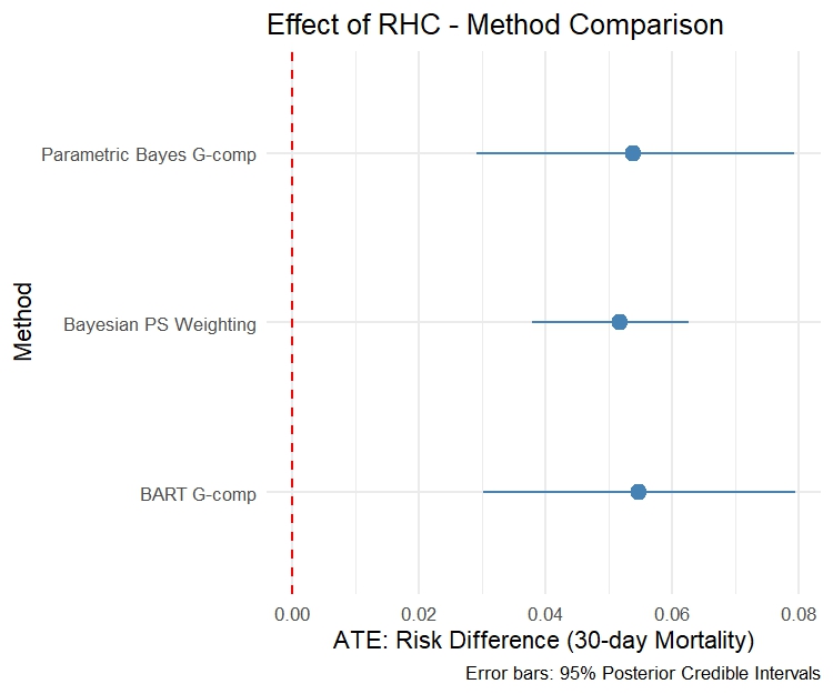
Comparing results from three methods

Method	Mean	2.5% CrI	97.5% CrI
Parametric Bayes G-comp	0.0537	0.0291	0.0792
BART G-comp	0.0546	0.0301	0.0794
Bayesian PS Weighting	0.0516	0.0379	0.0626

Part III: Time-Varying Treatments

Time-varying treatment and confounding

In many studies, treatment is assigned repeatedly over time and covariates measured between treatment occasions affect both future treatment and the outcome.

Notation

\(A_j\): binary treatment at visit \(j\)
\(L_j\): time-varying covariates at visit \(j\)
\(\bar{A}_j = (A_1,\ldots,A_j)\): treatment history up to \(j\)
\(\bar{L}_j = (L_1,\ldots,L_j)\): covariate history up to \(j\)
\(Y\): end-of-study outcome

For each treatment sequence \(\bar{a}\), the potential outcome is \(Y^{\bar{a}}\).

The causal estimand compares two sequences - e.g. always treated vs never treated: \(\Psi = E[Y^{\bar{a}=1}] - E[Y^{\bar{a}=0}]\)

The time-varying confounding problem

flowchart LR
  L0([L0]) --> A0([A0])
  L0 --> L1([L1])
  A0 --> L1
  L1 --> A1([A1])
  A0 --> A1
  L0 --> Y([Y])
  A0 --> Y
  L1 --> Y
  A1 --> Y

\(L_1\) is simultaneously:

A confounder of \(A_1 \to Y\) - must adjust for it
A mediator of \(A_0 \to Y\) - must not condition on it

Standard regression cannot handle both requirements simultaneously.

Marginal Structural Models are specifically designed for this setting.

Sequential ignorability

Key assumption: Sequential ignorability

At each visit \(j\), conditional on covariate and treatment history, treatment is independent of all future potential outcomes:

\[Y^{\bar{a}} \perp A_j \mid \{\bar{L}_j, \bar{A}_{j-1}\}, \quad j = 1, \ldots, J\]

This is the time-varying analogue of IA.1 - applied sequentially at each visit.

Positivity (time-varying)

At each visit, every treatment value has non-zero probability given any observed history:

\[P(A_j = a_j \mid \bar{L}_j, \bar{A}_{j-1}) > 0 \quad \forall\, a_j, \bar{l}_j, \bar{a}_{j-1}\]

Simulated longitudinal data

dat <- readr::read_csv("continuous_outcome_data.csv")
dplyr::glimpse(dat)

Two-visit study, \(n=1{,}000\), binary treatment, continuous outcome.

Variable	Description
`w1`, `w2`	Baseline covariates
`L1_1`, `L2_1`	Time-varying confounders, visit 1
`a_1`	Binary treatment, visit 1
`L1_2`, `L2_2`	Time-varying confounders, visit 2
`a_2`	Binary treatment, visit 2
`y`	Continuous end-of-study outcome

Bayesian MSMs: introduction

Instead of modelling the full confounder process (as in g-computation), MSMs model only the marginal potential outcome as a function of treatment history:

\[g_Y\Big(E[Y^{\bar{a}}]\Big) = \theta_0 + \Theta \sum_j A_j\]

\(\Theta\) is the causal effect of one additional treatment period - the marginal structural parameter.

MSMs use IPTW weighting to adjust for time-varying confounding - creating a pseudo-population where treatment is unconfounded.

The Bayesian approach (Saarela et al., 2015; Liu et al., 2020) derives MSM estimation from Bayesian decision theory - the same framework as Bayesian PS weighting, extended to the longitudinal setting.

Bayesian MSMs: estimation principle

The expected utility under the experimental distribution \(\mathcal{E}\): \[\hat{\Theta} \approx \underset{\Theta}{\operatorname{argmax}} \; \frac{1}{B}\sum_{b=1}^B \sum_{i=1}^n \pi_i^{(b)} \, \hat{w}_i \, \log P_{\mathcal{E}}(Y_i^* \mid \bar{A}_i^*;\, \Theta)\]

\(\pi^{(b)} \sim \text{Dir}_n(\mathbf{1})\) - Bayesian bootstrap weights over the observational distribution
\(\hat{w}_i\) - posterior mean stabilized IPTW weights from Bayesian treatment models
\(P_{\mathcal{E}}(Y \mid \bar{A};\, \Theta)\) - the marginal structural model likelihood

Two-step estimation

Step 1 (parametric): Fit Bayesian logistic regression models at each visit to get posterior IPTW weights \(\hat{w}_i\)

Step 2 (nonparametric): Maximise the weighted utility over \(B\) Bayesian bootstrap iterations for posterior distribution of \(\Theta\)

Bayesian MSM: weight estimation

library(bayesmsm)

bayes_wt <- bayesweight(
  trtmodel.list = list(
    a_1 ~ w1 + w2 + L1_1 + L2_1,
    a_2 ~ w1 + w2 + L1_1 + L2_1 + L1_2 + L2_2 + a_1),
  data     = dat,
  n.iter   = 2500, n.burnin = 1500, n.thin = 5,
  parallel = TRUE, n.chains = 2, seed = 42)

bayesweight() fits visit-specific Bayesian logistic regression models via JAGS and returns posterior mean stabilized weights for each subject. The package automatically generates the JAGS model file - which can be inspected and customized.

Bayesian MSM: outcome estimation

msm_fit <- bayesmsm(
  ymodel     = y ~ a_1 + a_2,
  family     = "gaussian",
  nvisit     = 2,
  reference  = c(0, 0),      # never treated
  comparator = c(1, 1),      # always treated
  data       = dat,
  wmean      = bayes_wt$weights,
  nboot      = 1000,
  optim_method = "BFGS",
  parallel   = TRUE, seed = 42)

Bayesian MSM: results

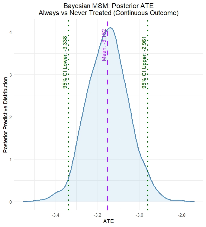
summary_bayesmsm(msm_fit)

plot_ATE(msm_fit,
         col_density = "steelblue",
         main = "Posterior ATE: Always vs Never Treated")

plot_ATE() displays the full posterior density of \(\Psi = E[Y^{\bar{a}=1}] - E[Y^{\bar{a}=0}]\) - the causal effect of always being treated versus never treated on the continuous outcome.

The posterior reflects uncertainty from both the treatment weight models (Step 1) and the Bayesian bootstrap over the outcome model (Step 2).

Bayesian MSM: results 2

	Mean	SD	2.5% CrI	97.5% CrI
Reference (never treated)	2.316	0.048	2.219	2.410
Comparator (always treated)	-0.836	0.076	-0.986	-0.685
Risk Difference	-3.152	0.098	-3.338	-2.961

Part IV: Bayesian Sensitivity Analysis

The core problem

All methods covered so far assume conditional ignorability (IA.1): \[Y^a \perp A \mid L\]

This assumption is untestable from observed data - we can never verify that all confounders are measured.

What if an unmeasured confounder \(U\) exists?

\(U\) affects both treatment assignment and the outcome - but is absent from \(L\). Standard analyses proceed as if IA.1 holds, producing potentially biased estimates.

The Bayesian advantage

Since the impact of unmeasured confounding is non-identifiable from data, the Bayesian framework treats it as just another unknown parameter - with a prior expressing our beliefs about its magnitude and direction.

Unmeasured confounding - a latent variable

Suppose an unmeasured confounder \(U\) exists such that \(A \not\perp Y^1, Y^0 \mid L\), but: \[A \perp Y^1, Y^0 \mid L, U\]

We model \(U\) as latent - treat it as missing data and sample it jointly with all model parameters. Assume conservatively: \[U \sim N(0,1), \quad U \perp L\]

\(U \perp L\) is conservative: if \(U\) were correlated with measured \(L\), adjusting for \(L\) would partially remove confounding.

Unmeasured confounding - ATE

Under this modified ignorability, the ATE is identified as: \[\Psi(\eta, \theta, \xi) = \iint \Big[E[Y \mid A=1, L=l, U=u;\, \eta, \xi] - E[Y \mid A=0, L=l, U=u;\, \eta, \xi]\Big]\] \[\times f_L(l;\theta)\,\phi(u)\, dl\, du\]

where \(\xi\) are sensitivity parameters - non-identifiable, governing dependence of outcome and treatment on \(U\).

Sensitivity parameters \(\xi_1\) and \(\xi_2\)

For binary outcome \(Y\) and binary treatment \(A\) with single confounder \(L\), specify:

\[P(Y=1 \mid a, l, u;\, \eta, \xi_1) = \text{expit}(\eta_0 + \eta_1 a + \eta_2 l + \xi_1 u)\] \[P(A=1 \mid l, u;\, \gamma, \xi_2) = \text{expit}(\gamma_0 + \gamma_1 l + \xi_2 u)\]

Interpretation:

\(\xi_1\): among patients with same \(A\) and \(L\), a 1 SD higher \(U\) multiplies the odds of \(Y\) by \(e^{\xi_1}\)
\(\xi_2\): among patients with same \(L\), a 1 SD higher \(U\) multiplies the odds of treatment by \(e^{\xi_2}\)
\(\xi_1 = \xi_2 = 0\): strong prior belief in no unmeasured confounding - the null values

Prior specification for bias parameters

Why this is a practical approach?

The latent \(U\) approach directly models the mechanism by which confounding operates - through both outcome and treatment models simultaneously.
The sensitivity parameters \(\xi_1\) and \(\xi_2\) have clear OR-scale interpretations. The posterior of \(\Psi\) automatically accounts for uncertainty in all \(U_i\) values.

Prior choices for \(\xi_1\), \(\xi_2\)

Prior	Encodes
\(\xi_1, \xi_2 \sim N(0, \sigma^2)\)	Symmetric uncertainty about confounding
Grid of point masses	Tipping point - trace posterior across \((\xi_1, \xi_2)\) values

Bayesian MCMC samples \(U_i\) for every subject at every MCMC iteration - treating the latent confounder values as additional parameters. This is the missing data framing: \(U\) is unknown, so we do posterior inference on it.

Sensitivity analysis: Stan model

data {
  int<lower=0> N;
  vector[N] Y;        // binary outcome (0/1 as real)
  vector[N] A;        // binary treatment
  vector[N] L;        // observed confounder
  real xi1;           // sensitivity parameter: U -> Y (fixed per grid point)
  real xi2;           // sensitivity parameter: U -> A (fixed per grid point)
}
parameters {
  real eta0; real eta1; real eta2;   // outcome model
  real gam0; real gam1;              // treatment model
  vector[N] U;                       // latent unmeasured confounder
}
model {
  // Priors
  eta0 ~ normal(0, 3); eta1 ~ normal(0, 3); eta2 ~ normal(0, 3);
  gam0 ~ normal(0, 3); gam1 ~ normal(0, 3);
  U    ~ normal(0, 1);               // U ~ N(0,1) standardized latent confounder

  // Likelihood - both outcome and treatment depend on U
  Y ~ bernoulli_logit(eta0 + eta1*A + eta2*L + xi1*U);
  A ~ bernoulli_logit(gam0 + gam1*L + xi2*U);
}
generated quantities {
  // G-computation ATE integrating over posterior U draws
  vector[N] mu1 = inv_logit(eta0 + eta1*1 + eta2*L + xi1*U);
  vector[N] mu0 = inv_logit(eta0 + eta1*0 + eta2*L + xi1*U);
  real psi = mean(mu1) - mean(mu0);
}

Sensitivity analysis: R code

library(rstan)

# Grid of (xi1, xi2) pairs to explore
xi_grid <- expand.grid(
  xi1 = c(0, 0.5, 1.0, 1.5, 2.0),
  xi2 = c(0, 0.5, 1.0, 1.5, 2.0))

stan_data_base <- list(
  N = nrow(rhc), Y = rhc$Y_death,
  A = rhc$A,     L = scale(rhc$age)[,1])

# Fit Stan model at each grid point
psi_grid <- lapply(1:nrow(xi_grid), function(k){
  d        <- c(stan_data_base,
                xi1 = xi_grid$xi1[k],
                xi2 = xi_grid$xi2[k])
  fit      <- sampling(sens_mod, data = d,
                       chains = 2, iter = 1500,
                       warmup = 500, seed = 42,
                       refresh = 0)
  psi_draws <- extract(fit, "psi")[[1]]
  data.frame(xi1  = xi_grid$xi1[k],
             xi2  = xi_grid$xi2[k],
             mean = mean(psi_draws),
             lo   = quantile(psi_draws, 0.025),
             hi   = quantile(psi_draws, 0.975))
}) |> dplyr::bind_rows()

Results

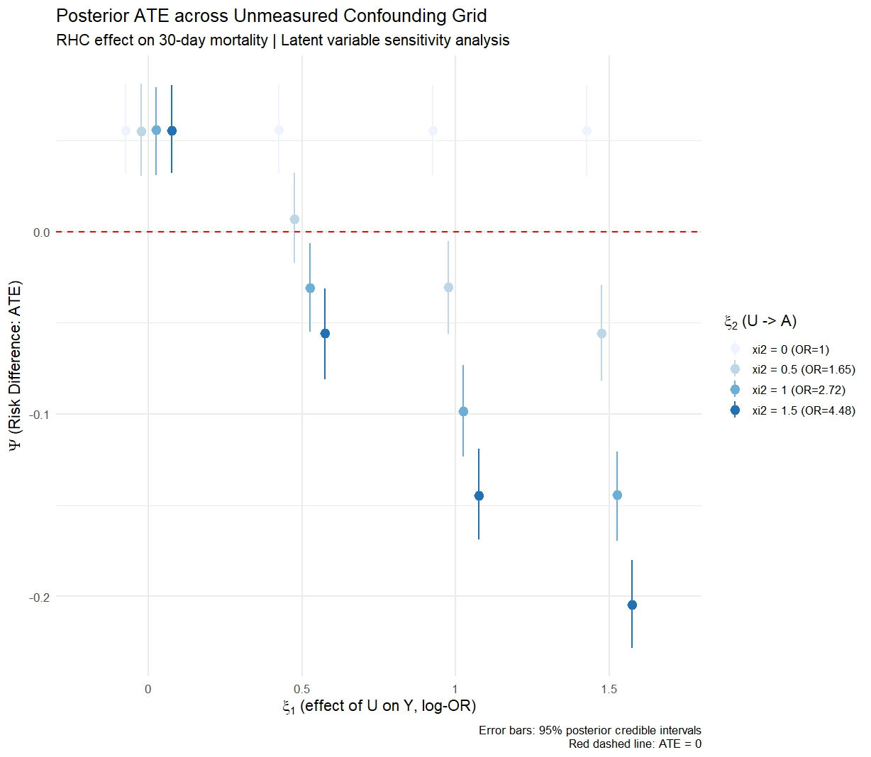
Tipping point: posterior ATE across \((\xi_1, \xi_2)\) grid

ggplot(psi_grid,
       aes(x = xi1, y = mean, ymin = lo, ymax = hi,
           colour = factor(xi2), group = factor(xi2))) +
  geom_pointrange(position = position_dodge(0.1)) +
  geom_hline(yintercept = 0, linetype = "dashed", colour = "red") +
  labs(x = expression(xi[1] ~ "(U -> Y, log-OR scale)"),
       y = expression(Psi ~ "(Risk Difference)"),
       colour = expression(xi[2] ~ "(U -> A)"),
       title = "Posterior ATE across unmeasured confounding grid",
       subtitle = "RHC effect on 30-day mortality") +
  theme_minimal(base_size = 13)

Tipping point heatmap

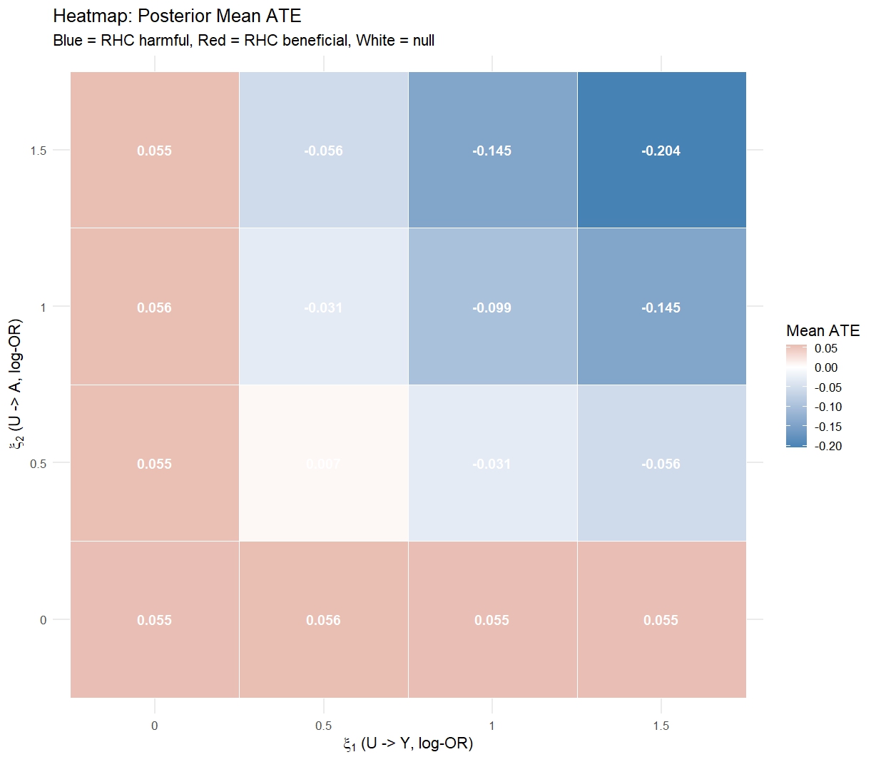
Reading the plot

The tipping point is the \((\xi_1, \xi_2)\) combination at which the 95% CrI crosses zero. If this requires \(e^{\xi_1} > 2\) or \(e^{\xi_2} > 2\) (i.e. \(U\) doubles the odds of both outcome and treatment), and subject-matter knowledge says this is implausible, the finding is robust.

Part V: Causal Forests & CATE

Motivation: treatment effect heterogeneity

The ATE \(\Psi = E[Y^1 - Y^0]\) is a single population summary - it hides potentially important variation in who benefits and who is harmed.

The Conditional Average Treatment Effect (CATE): \[\tau(x) = E[Y^1 - Y^0 \mid X = x]\]

answers: for a patient with characteristics \(x\), what is their expected treatment benefit?

CATE estimation enables:

Identifying subgroups that benefit most or are harmed
Personalizing treatment recommendations
Understanding effect modification

Bayesian Causal Forests: motivation

Naive BART for CATE: fit BART, compute \(\hat\tau(x) = \mu^{(m)}(1,x) - \mu^{(m)}(0,x)\).

Problem - regularization-induced confounding (Hahn et al., 2020):

The same BART prior shrinks both the prognostic effect of \(L\) and the treatment effect toward zero. When confounding is strong, this shrinkage conflates the two, biasing CATE estimates.

Solution - Bayesian Causal Forests (BCF):

Decompose the conditional mean into separate components with separate priors:

\[E[Y \mid A, x] = \underbrace{\mu(x, \hat{e}(x))}_{\text{prognostic (BART)}} + A \cdot \underbrace{\tau(x)}_{\text{treatment effect (BART)}}\]

\(\mu(x)\) uses a standard BART prior, captures the baseline prognosis and absorbs confounding via \(\hat{e}(x)\)

BCF: propensity score inclusion

BCF includes the estimated propensity score \(\hat{e}(x)\) directly in \(\mu(x)\):

\[\mu(x) = f(x, \hat{e}(x))\]

Why? Including \(\hat{e}(x)\) in the prognostic function allows the model to:

Absorb confounding into \(\mu(x)\) rather than \(\tau(x)\)
Let \(\tau(x)\) focus on treatment effect variation
Reduce bias from regularization-induced confounding

The posterior over \(\tau(x_i)\) gives:

Subject-level CATE estimates with full uncertainty quantification
Posterior probability \(P(\tau(x_i) > 0 \mid \mathcal{D})\) for each individual

BCF: fitting the model

library(bcf)

covars <- c("age","sex","race","cat1",
            "meanbp1","hrt1","resp1","temp1","wtkilo1")
X <- model.matrix(~ ., data = rhc[, covars])[, -1]
Y <- rhc$Y_death
A <- rhc$A

# Step 1: Estimate propensity scores
ps_fit <- glm(A ~ ., data = data.frame(A, X), family = binomial)
ps_hat <- fitted(ps_fit)

# Step 2: Fit BCF
bcf_fit <- bcf(
  y          = Y,
  z          = A,
  x_control  = X,       # enters mu(x)
  x_moderate = X,       # enters tau(x)
  pihat      = ps_hat,  # included in mu(x)
  nburn = 500, nsim = 1000, seed = 42)

BCF: posterior CATE draws

# Posterior CATE: n_subjects x n_draws matrix
tau_draws <- bcf_fit$tau

tau_hat <- rowMeans(tau_draws)
tau_lo  <- apply(tau_draws, 1, quantile, 0.025)
tau_hi  <- apply(tau_draws, 1, quantile, 0.975)

# Posterior probability of benefit for each subject
prob_benefit <- rowMeans(tau_draws > 0)

tau_draws contains the full posterior distribution over \(\tau(x_i)\) for every subject - not just a point estimate. This enables individual-level probabilistic statements about treatment benefit.

BCF: CATE by age subgroup

cate_df <- data.frame(
  tau_hat = tau_hat, tau_lo = tau_lo, tau_hi = tau_hi,
  age_q   = cut(rhc$age, quantile(rhc$age, 0:4/4),
                labels = c("Q1 (youngest)","Q2","Q3","Q4 (oldest)"),
                include.lowest = TRUE))
cate_sub <- cate_df |>
  group_by(age_q) |>
  summarise(mean = mean(tau_hat), lo = mean(tau_lo), hi = mean(tau_hi))

Age Group	Mean CATE	2.5% CrI	97.5% CrI	P(benefit)
Q1 (youngest)	0.0514	0.0011	0.1066	0.970
Q2	0.0485	-0.0015	0.0997	0.964
Q3	0.0481	-0.0010	0.0973	0.965
Q4 (oldest)	0.0474	-0.0009	0.0956	0.966

Summary

What we covered

Method	Package used in this tutorial
Parametric Bayes g-comp	`rstanarm`
NP Bayes g-comp (BART)	`BART`
Bayes PS weighting	`rstanarm` + Stan
Bayesian MSM	`bayesmsm`
Bayes sensitivity analysis	Stan
Causal forests (BCF)	`bcf`

Selected references

Oganisian & Roy (2021). A practical introduction to Bayesian estimation of causal effects. Statistics in Medicine, 40(2).
Saarela et al. (2015). On Bayesian estimation of marginal structural models. Biometrics, 71(2).
Liu et al. (2020). Estimation of causal effects with repeatedly measured outcomes in a Bayesian framework. Statistical Methods in Medical Research, 29(9).
Hahn, Murray & Carvalho (2020). Bayesian regression tree models for causal inference. Bayesian Analysis, 15(3).

Selected references

Oganisian (2026). Stress-Testing Assumptions: A Guide to Bayesian Sensitivity Analyses in Causal Inference. arXiv:2602.23640.
Chipman, George & McCulloch (2010). BART: Bayesian additive regression trees. AOAS, 4(1).
Rubin (1981). The Bayesian bootstrap. Annals of Statistics, 9(1).
Connors, A. F., Speroff, T., Dawson, N. V., Thomas, C., Harrell, F. E., Wagner, D., … & Knaus, W. A. (1996). The effectiveness of right heart catheterization in the initial care of critically III patients. JAMA, 276(11).