# install.packages(tidyverse, dependencies = T)
library(tidyverse) # load package library1. Getting started with R
Learning Objectives
- learn about R and RStudio work environment
- use R as a calculator
- understand objects in R
- learn about simple iterative programming in R
1.1 R and RStudio
R is a language and environment for statistical computing and graphics (https://cran.r-project.org/manuals.html).
Many users of R like to use RStudio as the preferred interface for programming in R.
RStudio is an Integrated Development Environment (IDE) for R.
- easy to navigate
- lots of point and click features and customizations
- Rstudio is not just for R
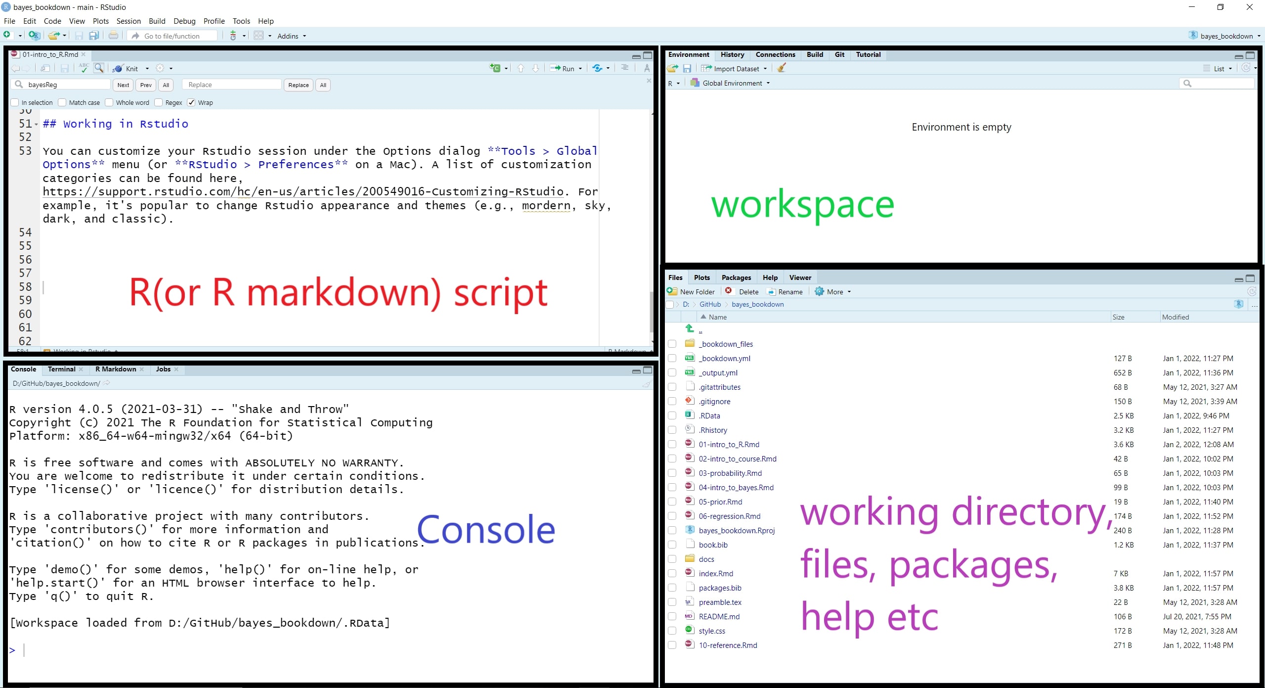
RStudio layout
When you open RStudio, your interface is made up of four panes as shown below. These can be organised via menu options View > Panes >
R Packages
Packages are the fundamental units of reproducible R code.
They include reusable R functions, the documentation that describes how to use them, and sample data.
We install the package using
install.packages()function or we can use the Package tab in Rstudio.Once we have the package installed, we must load the functions from this library so we can use them within R.
R script
We can run code in the console at the prompt where R will evaluate it and print the results.
best practice write code in a new script file so it can be saved, edited, and reproduced.
To open a new script, we select File > New File > R Script.
To “run code” that was written in the script file, you can highlight the code lines you wish be evaluated and
- press CTRL-Enter (windows)
- Cmd+Return (Mac).
Additionally, You can comment or uncomment script lines by pressing
- Ctrl+Shift+C (windows)
- Cmd+Shift+C (Mac).
The comment operator in R is
#.You can find more RStudio default keyboard shortcuts here.
Customization
You can customize your RStudio session under the Options dialog Tools > Global Options menu (or RStudio > Preferences on a Mac).
A list of customization categories can be found here.
Working directory
The working directory is the default location where R will look for files you want to load and where it will put any files you save.
You can use function
getwd()to display your current working directoryand use function
setwd()to set your working directory to a new folder on your computer.
getwd() #show my current working directory;[1] "D:/GitHub/Rworkshop"Getting help with R
The help section of R is extremely useful if you need more information about the packages and functions that you are currently loaded.
You can initiate R help using the help function
help()or?, the help operator.
help(ggplot)1.2 Basic R
- In this subsection, I will briefly outline some common R functions and commands for arithmetic, creating and working with objects such as vector and matrix
R is case sensitive.
Commands are separated by a newline in the console.
The # character can be used to make comments. R does not execute the rest of the line after the # symbol - it ignores it.
Previous commands can be accessed via the up and down arrow keys on the keyboard.
When naming in R, avoid using spaces and special characters (i.e., !@#$%^&*()_+=;:’“<>?/) and avoid leading names with numbers.
it’s common to see error and warning messages pop up as output in Console
- best solution: searching for online answers!
Arithmetic
2+3
3-2
2*3
2^3
3/2
2 + (2 + 3) * 2 - 5pi[1] 3.141593exp(1)[1] 2.718282exp(3)[1] 20.08554log(exp(1), base = exp(1)) #playing with Euler's number;[1] 1log(3, base = exp(1)) #default natural logarithms;[1] 1.098612log(3, base = 10)[1] 0.4771213log10(3)[1] 0.4771213log(-1) #warning message;[1] NaN- Some of the other available useful functions are:
abs(), sqrt(), ceiling(), floor(), trunc(), round().
Working with objects
R is an object-oriented programming language.
We can create objects and save them in our workspace & environment
An object is composed of three parts: 1) a value we’re interested in 2) an identifier and 3) the assignment operator.
Value: can take any forms
- a number, a string of characters, a data frame, a plot or a function
identifier is the name you assign to the value.
assignment operator resembles an arrow
<-and is used to link the value to the identifier.
# Creating a scalar called "a" and assigning a value of 2
a<-2

# Creating a scalar called "b" and assigning a value of 3
b<-3

# Adding "a" and "b" and saving under "d"
d<-a+b

# Printing the value of "d"
d
[1] 5# Updating the value of a scalar
# Adds 5 to the old value of "a" and saves it again under the name "a".
a<-a+5
a[1] 7Logic check
- TRUE or FALSE?
| Operator | |
|---|---|
| == | exactly equal to |
| != | not equal to |
| < | less than |
| <= | less than or equal to |
| > | greater than |
| >= | greater than or equal to |
| x | y | x or y |
| x & y | x and y |
a<5   # checks if x is less than 5 or not
a>5   # checks if x is greater than 5 or not
a<=5  # less or equal
a>=5  # greater or equal
a==4   #( == stands for equal)
a!=4   #( != stands for not equal)
Data structures
- Vectors
- Matrices
- arrays
- Data frames
- List
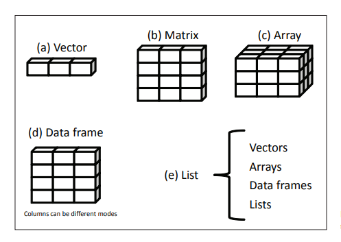
Vectors
vectors can contain same type or mixed type elements.
vector.name <- c(value1, value2, value3, ...).The function
c()means combine or concatenate and is used to create vectors.Types of elements:
- numeric(double)
- integer
- character
- logical: TRUE, FALSE
- Special values: NA(not available or missing), NULL(empty), NaN(not a number), Inf(infinite)
You can use
typeof()orclass()to examine an object’s type, or use anis()function.
# a vector of a single numeric element;
x <- 3
x
[1] 3typeof(x) #also try class(x);[1] "double"is(x)[1] "numeric" "vector" # a character vector
x <- c("red", "green", "yellow")
x[1] "red" "green" "yellow"typeof(x) #also try class(x);[1] "character"length(x)[1] 3nchar(x) #number of characters for each element;[1] 3 5 6# encode a vector as a factor (or category);
y <- factor(c("red", "green", "yellow", "red", "red", "green"))
y[1] red green yellow red red green
Levels: green red yellowattributes(y)$levels
[1] "green" "red" "yellow"
$class
[1] "factor"as.numeric(y) # we can return factors with numeric labels;[1] 2 1 3 2 2 1# we can update the levels;
levels(y)<- c("green","yellow","red")
attributes(y)$levels
[1] "green" "yellow" "red"
$class
[1] "factor"# we can also label numeric vector with factor levels;
z <- factor(c(1,2,3,1,1,2), levels = c(1,2,3), labels = c("red", "green","yellow"))
z[1] red green yellow red red green
Levels: red green yellowattributes(z)$levels
[1] "red" "green" "yellow"
$class
[1] "factor"# using the repeat command;
# the following line repeats 3, 5 times
rep(x=3,each=5) [1] 3 3 3 3 3# using sequence command;
1:10 [1] 1 2 3 4 5 6 7 8 9 10seq(from=1, to=10, by=1) [1] 1 2 3 4 5 6 7 8 9 10rep(x=1:2, each = 2)[1] 1 1 2 2- Logical check for a vector
- Just like a scalar, we can evaluate logical conditions using a vector as well.
- This is an element-wise operation.
- R will check every element of the vector
- The output will be a TRUE/FALSE vector.
#Let's star with a new vector which has 5 elements
x<- c(3,6,2,8,10)
x>5
[1] FALSE TRUE FALSE TRUE TRUEx==2[1] FALSE FALSE TRUE FALSE FALSEsum(x>5)[1] 3- select or remove elements from a vector
- we use the open bracket
[ ]after the vector and use index to operate.
- we use the open bracket
#Starting with same x vector
# x= c(3,6,2,8,10)

x[1]          # gives us the first element
[1] 3x[c(1,3,4) ] # return the 1st, 3rd and 4th element[1] 3 2 8x[-1] # remove the first element[1] 6 2 8 10x[-1:-2] # remove first and second elements[1] 2 8 10x[-c(1,2)][1] 2 8 10- Calculating summary statistics of a vector
set.seed(123)
r <- sample(x = 1:100, size = 100, replace = TRUE)
mean(r)  #calculate the mean of a vector
[1] 52.15var(r) #variance of a vector[1] 874.7348sd(r) #standard deviation of a vector[1] 29.57592min(r) #minimum of a vector[1] 4max(r) #maximum of a vector[1] 99median(r)#median[1] 50range(r) #range[1] 4 99Matrices
- matrices have two dimensions, rows and columns
# matrix in R;
matrix(data = 1:16, nrow=4, ncol=4, byrow=TRUE)
[,1] [,2] [,3] [,4]
[1,] 1 2 3 4
[2,] 5 6 7 8
[3,] 9 10 11 12
[4,] 13 14 15 16matrix(data = 1:16, nrow=4, ncol=4, byrow=FALSE) [,1] [,2] [,3] [,4]
[1,] 1 5 9 13
[2,] 2 6 10 14
[3,] 3 7 11 15
[4,] 4 8 12 16# creating matrix using diagonal;
diag(c(1,1,1)) [,1] [,2] [,3]
[1,] 1 0 0
[2,] 0 1 0
[3,] 0 0 1# matrix calculation;
X <- matrix(data = 1:16, nrow=4, ncol=4, byrow=TRUE)
diag(X)[1] 1 6 11 16t(X) #transpose; [,1] [,2] [,3] [,4]
[1,] 1 5 9 13
[2,] 2 6 10 14
[3,] 3 7 11 15
[4,] 4 8 12 16Y <- matrix(seq(1,32, by=2), nrow=4, byrow=T)
Y [,1] [,2] [,3] [,4]
[1,] 1 3 5 7
[2,] 9 11 13 15
[3,] 17 19 21 23
[4,] 25 27 29 31# matrix operation;
Y + X [,1] [,2] [,3] [,4]
[1,] 2 5 8 11
[2,] 14 17 20 23
[3,] 26 29 32 35
[4,] 38 41 44 47Y - X [,1] [,2] [,3] [,4]
[1,] 0 1 2 3
[2,] 4 5 6 7
[3,] 8 9 10 11
[4,] 12 13 14 153 * X [,1] [,2] [,3] [,4]
[1,] 3 6 9 12
[2,] 15 18 21 24
[3,] 27 30 33 36
[4,] 39 42 45 48X * Y [,1] [,2] [,3] [,4]
[1,] 1 6 15 28
[2,] 45 66 91 120
[3,] 153 190 231 276
[4,] 325 378 435 496X %*% Y #inner product; [,1] [,2] [,3] [,4]
[1,] 170 190 210 230
[2,] 378 430 482 534
[3,] 586 670 754 838
[4,] 794 910 1026 1142Data frames
A data frame is a group of vectors of the same length.
Two dimensions: columns are variables and rows are observations
Unlike matrix, a data frame can contain different data types (e.g., numeric or character)
site_id <- c("A", "B", "C", "D")  #identifies the soil sampling site;
soil_pH <- c(6.1, 7.4, 5.1, 6)  #soil pH
num_species <- c(17, 23, 7, 15)  #number of species
treated <- c("yes", "yes", "no", "no")  #treatment status;

# use data.frame function to create a data frame;
soil_data <- data.frame(site_id, soil_pH, num_species, treated)

# view data;
soil_data
site_id soil_pH num_species treated
1 A 6.1 17 yes
2 B 7.4 23 yes
3 C 5.1 7 no
4 D 6.0 15 nostr(soil_data)'data.frame': 4 obs. of 4 variables:
$ site_id : chr "A" "B" "C" "D"
$ soil_pH : num 6.1 7.4 5.1 6
$ num_species: num 17 23 7 15
$ treated : chr "yes" "yes" "no" "no"dim(soil_data)[1] 4 4nrow(soil_data)[1] 4ncol(soil_data)[1] 4colnames(soil_data)[1] "site_id" "soil_pH" "num_species" "treated" Lists
- highly flexible objects
- lists can contain anything as their elements
example_list <- list(
  num = sep(from=1, to=10, by=2),
  char = c("apple", "pineapple"),
  logic = c(TRUE, TRUE, FALSE)
)
1.3 Advanced topics - iterative programming
if statements in R
- If statements in R has got this following structure
if (condition){expression}
A simple example:
x<-3
if(x==3){print("x is 3")}
[1] "x is 3"if else statement
if(condition){
  expression1
  } else {
  expression2
}- we can also use
ifelse()function,ifelse(condition, expression 1, expression 2)
y <- c(6:-4)
sqrt(y)  #- gives warning
Warning in sqrt(y): NaNs produced [1] 2.449490 2.236068 2.000000 1.732051 1.414214 1.000000 0.000000 NaN
[9] NaN NaN NaNsqrt(ifelse(y >= 0, x, NA)) # no warning [1] 1.732051 1.732051 1.732051 1.732051 1.732051 1.732051 1.732051 NA
[9] NA NA NAmultiple conditions
if (condition1) {
    expression1
} else if (condition2) {
    expression2
} else if (condition3) {
    expression3
} else {
    expression4
}
# current value of x is 3
if(x==4){
print("x is 4")
}else if (x>4){
print("x is greater than 4")
}else if (x<4){
print("x is less than 4")
}[1] "x is less than 4"For Loops
- perform a particular action for every iteration of some sequence
for (i in sequence){
  expression
}- a simple example
for (month in 1:12) {
    print(paste('Month:', month))
}
[1] "Month: 1"
[1] "Month: 2"
[1] "Month: 3"
[1] "Month: 4"
[1] "Month: 5"
[1] "Month: 6"
[1] "Month: 7"
[1] "Month: 8"
[1] "Month: 9"
[1] "Month: 10"
[1] "Month: 11"
[1] "Month: 12"- a slightly more complex example combining for loop and if statements - counting even numbers
x <- c(2,5,3,9,8,11,6)
count <- 0
for (val in x) {
if(val %% 2 == 0)  count = count+1
}
print(count)
[1] 3apply family
apply family functions can be used in the same way as a for loop
apply()- apply over the margins of an array (e.g. the - rows or columns of a matrix)
lapply()- apply over an object and return list
sapply()- apply over an object and return a simplified object (an array) if possible
vapply()- similar to sapply but you specify the type of object returned by the iterations
mapply()- multivariate version of
sapply()
- multivariate version of
tapply()- used to apply a function over subsets of a vector
# a matrix with apply;
mymatrix<-matrix(1:9,nrow=3)
mymatrix
[,1] [,2] [,3]
[1,] 1 4 7
[2,] 2 5 8
[3,] 3 6 9# calculate row sum;
apply(X=mymatrix,MARGIN=1,FUN = sum) [1] 12 15 18# a list with lapply
mylist<-list(A=matrix(1:9,nrow=3),B=1:5,C=8)
# calculate sum for each element of the list;
lapply(mylist,FUN = sum)$A
[1] 45
$B
[1] 15
$C
[1] 8# calculate sum for each element of the list and simplify it to a vector;
sapply(mylist, FUN = sum) A B C
45 15 8
Tips
Where possible, use vectorized operations instead of for loops to make code faster and more concise.
Use functions such as apply instead of for loops to operate on the values in a data structure.
Effectively use loops in statistically modelling
This can be handy in statistical modelling!
Data: Motor Trend Car Road Tests
- A data frame with 32 observations on 11 (numeric) variables.
- mpg Miles/(US) gallon
- cyl Number of cylinders
- disp Displacement (cu.in.)
- hp Gross horsepower
- drat Rear axle ratio
- wt Weight (1000 lbs)
- qsec 1/4 mile time
- vs Engine (0 = V-shaped, 1 = straight)
- am Transmission (0 = automatic, 1 = manual)
- gear Number of forward gears
- carb Number of carburetors
- A data frame with 32 observations on 11 (numeric) variables.
library(DT)
datatable(mtcars,
          options = list(dom = 't'))
# creating a list a variables that are predictive of the fuel consumption;
predictors <- colnames(mtcars)[-1]
predictors [1] "cyl" "disp" "hp" "drat" "wt" "qsec" "vs" "am" "gear" "carb"#run unadjusted regression analysis for each predictor;
# m1 <- lm(mpg~cyl,data = mtcars)
# m2 <- lm(mpg~disp,data = mtcars)
# m3 <- lm(mpg~hp,data = mtcars)
# make a list of model formulars: list(mpg ~ cyl, mpg ~ disp, ...);
list_model_formulas <- sapply(predictors,function(x)as.formula(paste('mpg~',x)))
# making a list of unadjusted models;
list_models <- lapply(list_model_formulas,function(x){lm(x,data=mtcars)})
#extract model results;
results <- lapply(list_models, function(x){return(summary(x)$coef)})
results$cyl
Estimate Std. Error t value Pr(>|t|)
(Intercept) 37.88458 2.0738436 18.267808 8.369155e-18
cyl -2.87579 0.3224089 -8.919699 6.112687e-10
$disp
Estimate Std. Error t value Pr(>|t|)
(Intercept) 29.59985476 1.229719515 24.070411 3.576586e-21
disp -0.04121512 0.004711833 -8.747152 9.380327e-10
$hp
Estimate Std. Error t value Pr(>|t|)
(Intercept) 30.09886054 1.6339210 18.421246 6.642736e-18
hp -0.06822828 0.0101193 -6.742389 1.787835e-07
$drat
Estimate Std. Error t value Pr(>|t|)
(Intercept) -7.524618 5.476663 -1.373942 0.1796390847
drat 7.678233 1.506705 5.096042 0.0000177624
$wt
Estimate Std. Error t value Pr(>|t|)
(Intercept) 37.285126 1.877627 19.857575 8.241799e-19
wt -5.344472 0.559101 -9.559044 1.293959e-10
$qsec
Estimate Std. Error t value Pr(>|t|)
(Intercept) -5.114038 10.0295433 -0.5098974 0.61385436
qsec 1.412125 0.5592101 2.5252133 0.01708199
$vs
Estimate Std. Error t value Pr(>|t|)
(Intercept) 16.616667 1.079711 15.389917 8.846603e-16
vs 7.940476 1.632370 4.864385 3.415937e-05
$am
Estimate Std. Error t value Pr(>|t|)
(Intercept) 17.147368 1.124603 15.247492 1.133983e-15
am 7.244939 1.764422 4.106127 2.850207e-04
$gear
Estimate Std. Error t value Pr(>|t|)
(Intercept) 5.623333 4.916379 1.143796 0.261753365
gear 3.923333 1.308131 2.999191 0.005400948
$carb
Estimate Std. Error t value Pr(>|t|)
(Intercept) 25.872334 1.8368072 14.08549 9.218370e-15
carb -2.055719 0.5685456 -3.61575 1.084446e-03