2. Working with Data

Published

2023-01-12

Learning Objectives

Loading, exploring and saving data
Learn to manipulate data frames with tidyverse
Overview of ggplot2 for data visualization

For this session, we will be working with the co2_mm_gl_clean.csv dataset
This data contains monthly globally averaged CO2 records between 1979 and 2022.
Lan, X., Tans, P. and K.W. Thoning: Trends in globally-averaged CO2 determined from NOAA Global Monitoring Laboratory measurements. Version 2023-01 NOAA/GML (https://gml.noaa.gov/ccgg/trends/)

2.1 Data import and export

package readr reads txt, csv, Rdata (or rda).
package haven reads SPSS, Stata, and SAS files.
package readxl reads excel files (both .xls and .xlsx).

library(tidyverse)
knitr::opts_chunk$set(echo = TRUE, fig.align="center")
options(scipen = 999, pillar.print_max = Inf)
co2 <- read_csv(file = "co2_mm_gl_clean.csv")

Looking at the data

co2	Look at the whole data frame
head(co2)	Look at the first few rows
tail(co2)	Look at the last few rows
colnames(co2)	Names of the columns in the data frame
attributes(co2)	Attributes of the data frame
dim(co2)	Dimensions of the data frame
ncol(co2)	Number of columns
nrow(co2)	Number of rows
summary(co2)	Summary statistics
str(co2)	Structure of the data frame

library(DT)
datatable(co2)

str(co2)

spc_tbl_ [526 × 5] (S3: spec_tbl_df/tbl_df/tbl/data.frame)
 $ year   : num [1:526] 1979 1979 1979 1979 1979 ...
 $ month  : num [1:526] 1 2 3 4 5 6 7 8 9 10 ...
 $ decimal: num [1:526] 1979 1979 1979 1979 1979 ...
 $ average: num [1:526] 337 337 338 338 338 ...
 $ stddev : num [1:526] 0.1 0.09 0.1 0.11 0.04 0.17 0.27 0.29 0.2 0.22 ...
 - attr(*, "spec")=
  .. cols(
  ..   year = col_double(),
  ..   month = col_double(),
  ..   decimal = col_double(),
  ..   average = col_double(),
  ..   stddev = col_double()
  .. )
 - attr(*, "problems")=<externalptr>

summary(co2)

      year          month           decimal        average     
 Min.   :1979   Min.   : 1.000   Min.   :1979   Min.   :334.4  
 1st Qu.:1989   1st Qu.: 3.250   1st Qu.:1990   1st Qu.:353.2  
 Median :2000   Median : 6.000   Median :2001   Median :369.7  
 Mean   :2000   Mean   : 6.481   Mean   :2001   Mean   :372.6  
 3rd Qu.:2011   3rd Qu.: 9.000   3rd Qu.:2012   3rd Qu.:391.3  
 Max.   :2022   Max.   :12.000   Max.   :2023   Max.   :418.5  
     stddev       
 Min.   :0.03000  
 1st Qu.:0.08000  
 Median :0.10000  
 Mean   :0.09894  
 3rd Qu.:0.11000  
 Max.   :0.29000

Renaming variables

colnames(co2)[5]

[1] "stddev"

colnames(co2)[5] <- "sd"
colnames(co2)

[1] "year"    "month"   "decimal" "average" "sd"

Creating new variables

co2$lowerbound_1sd <- co2$average - 1*co2$sd
co2$upperbound_1sd <- co2$average + 1*co2$sd
head(co2)

# A tibble: 6 × 7
   year month decimal average    sd lowerbound_1sd upperbound_1sd
  <dbl> <dbl>   <dbl>   <dbl> <dbl>          <dbl>          <dbl>
1  1979     1   1979.    337.  0.1            336.           337.
2  1979     2   1979.    337.  0.09           337.           337.
3  1979     3   1979.    338.  0.1            338.           338.
4  1979     4   1979.    338.  0.11           338.           338.
5  1979     5   1979.    338.  0.04           338.           338.
6  1979     6   1979.    337.  0.17           337.           338.

Subsetting data

# extracting data between 2020 and 2022;
co2_2020_2022 <- subset(co2, year >= 2020 & year <=2022)

# subletting directly from dataframe using index;
# try at home;
# co2_2020_2022 <- CO2[CO2year >= 2020 & year <=2022, ]  # Select observations with year between 2020 and 2022;

we can export data from r using write function

write.csv(co2, file = 'co2_mm_gl_clean2.csv')

2.2 Data manipulation with tidyverse (a crush introduction)

What is the Tidyverse?

The tidyverse consists of a few key packages: - dplyr: data manipulation - ggplot2: data visualization - tibble: tibbles, a modern re-imagining of data frames - tidyr: data tidying - readr: data import - purrr: functional programming, e.g. alternate approaches to apply

Pipe operator %>%
Pipes are operators that send what comes before the pipe to what comes after.
frequently used in tidyverse!

Selecting Columns

Example: using %>% to subset data
- select() in dplyr subset columns by names
- filter() subset rows using column values

# selecting columns;
co2 %>%
  select(year, month, average) %>%
  head()

# drop some variables;
co2 %>%
  select(-month) %>%
  head()

Sometimes, we have a lot of variables to select, and if they have a common naming scheme, this can be very easy.

co2 %>%
  select(contains("bound")) %>%
  head()

Over helpful functions to be used within select()
- starts_with: starts with a prefix
- ends_with: ends with a suffix
- contains: contains a literal string
- matches: matches a regular expression
- num_range: a numerical range like wk1, wk2, wk3.
  - select(num_range("wk", 1:3))
- everything: all variables.

selecting rows

# selecting observations in year 2022;
co2 %>%
  select(year, month, average) %>%
  filter(year == 2022)

# A tibble: 10 × 3
    year month average
   <dbl> <dbl>   <dbl>
 1  2022     1    417.
 2  2022     2    418.
 3  2022     3    418.
 4  2022     4    418.
 5  2022     5    418.
 6  2022     6    417.
 7  2022     7    416.
 8  2022     8    414.
 9  2022     9    415.
10  2022    10    416.

# selecting observations between 2020 and 2022;
co2 %>%
  select(year, month, average) %>%
  filter(year <= 2022 & year >= 2020)

creating new variables

Example: using %>% and mutate() to create new variable

co2 %>%
  mutate(lowerbound_2sd = average - 2*sd,
         upperbound_2sd = average + 2*sd) %>%
  head()

# A tibble: 6 × 9
   year month decimal average    sd lowerbound_1sd upperbound_…¹ lower…² upper…³
  <dbl> <dbl>   <dbl>   <dbl> <dbl>          <dbl>         <dbl>   <dbl>   <dbl>
1  1979     1   1979.    337.  0.1            336.          337.    336.    337.
2  1979     2   1979.    337.  0.09           337.          337.    337.    337.
3  1979     3   1979.    338.  0.1            338.          338.    338.    338.
4  1979     4   1979.    338.  0.11           338.          338.    338.    339.
5  1979     5   1979.    338.  0.04           338.          338.    338.    338.
6  1979     6   1979.    337.  0.17           337.          338.    337.    338.
# … with abbreviated variable names ¹upperbound_1sd, ²lowerbound_2sd,
#   ³upperbound_2sd

# creating new variables based on conditions of another variable;
# suppose we want to create a year group variable;

co2 %>% 
  mutate(year_group = case_when(
    year < 1980 ~ '1970-1979',
    1980 <= year & year < 1990 ~ '1980-1989',
    1990 <= year & year < 2000 ~ '1990-1999',
    2000 <= year & year < 2010 ~ '2000-2009',
    2010 <= year & year < 2020 ~ '2010-2019',
    2020 <= year & year < 2030 ~ '2020-2029',
  )) %>%
  head()

# A tibble: 6 × 8
   year month decimal average    sd lowerbound_1sd upperbound_1sd year_group
  <dbl> <dbl>   <dbl>   <dbl> <dbl>          <dbl>          <dbl> <chr>     
1  1979     1   1979.    337.  0.1            336.           337. 1970-1979 
2  1979     2   1979.    337.  0.09           337.           337. 1970-1979 
3  1979     3   1979.    338.  0.1            338.           338. 1970-1979 
4  1979     4   1979.    338.  0.11           338.           338. 1970-1979 
5  1979     5   1979.    338.  0.04           338.           338. 1970-1979 
6  1979     6   1979.    337.  0.17           337.           338. 1970-1979

co2 <- co2 %>% #updating the data object
  mutate(year_group = case_when(
    year < 1980 ~ '1970-1979',
    1980 <= year & year < 1990 ~ '1980-1989',
    1990 <= year & year < 2000 ~ '1990-1999',
    2000 <= year & year < 2010 ~ '2000-2009',
    2010 <= year & year < 2020 ~ '2010-2019',
    2020 <= year & year < 2030 ~ '2020-2029',
  ))

Grouping and Summarizing Data

we can use group_by() and summarize() to help calculating group-based statistics
Example: suppose we want to calculate average, min, and max co2 by years (aggregated over month)

co2 %>%
  select(year, average) %>%
  group_by(year) %>%
  summarise(
    `mean co2 by month` = mean(average),
    `min co2 by month` = min(average),
    `max co2 by month` = max(average)
  )

# A tibble: 44 × 4
    year `mean co2 by month` `min co2 by month` `max co2 by month`
   <dbl>               <dbl>              <dbl>              <dbl>
 1  1979                337.               334.               338.
 2  1980                339.               337.               340.
 3  1981                340.               338.               342.
 4  1982                341.               338.               343.
 5  1983                343.               341.               344.
 6  1984                344.               342.               345.
 7  1985                346.               343.               347.
 8  1986                347.               345.               348.
 9  1987                349.               347.               350.
10  1988                351.               349.               352.
11  1989                353.               350.               354.
12  1990                354.               352.               356.
13  1991                355.               353.               357.
14  1992                356.               354.               358.
15  1993                357.               354.               358.
16  1994                358.               356.               360.
17  1995                360.               358.               362.
18  1996                362.               360.               363.
19  1997                363.               360.               365.
20  1998                366.               364.               367.
21  1999                368.               365.               369.
22  2000                369.               367.               370.
23  2001                371.               368.               372.
24  2002                373.               370.               374.
25  2003                375.               373.               377.
26  2004                377.               374.               378.
27  2005                379.               377.               381.
28  2006                381.               378.               383.
29  2007                383.               380.               384.
30  2008                385.               383.               387.
31  2009                386.               384.               388.
32  2010                389.               386.               390.
33  2011                391.               388.               392.
34  2012                393.               390.               394.
35  2013                395.               393.               397.
36  2014                397.               395.               399.
37  2015                400.               397.               402.
38  2016                403.               401.               405.
39  2017                405.               403.               407.
40  2018                408.               405.               409.
41  2019                410.               408.               412.
42  2020                412.               410.               414.
43  2021                415.               412.               417.
44  2022                417.               414.               418.

we observe an increasing trend of global co2 concenration over years.

Renaming columns

#example syntax;
data %>%
  rename(new_name = oldname,
         new_name2 = oldname2)

Reshaping datasets - wide vs long data

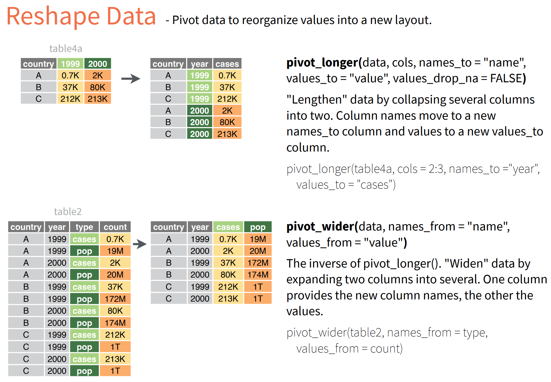R cheetsheet on reshaping data - pivot function has three argumnets:

The function requires the following arguments - a data frame (e.g. “wide”) - cols: name of the columns we wish to gather - names_to: name of the new column - values_to: name of the new column containing variable values

suppose we want to reshape the long co2 data to wide data with month 1 to 12 as columns

co2_wide <- co2 %>%
  select(year, month, average) %>%
  pivot_wider(names_from = month,
              names_prefix = "mth",
              values_from = average)

head(co2_wide)

# A tibble: 6 × 13
   year  mth1  mth2  mth3  mth4  mth5  mth6  mth7  mth8  mth9 mth10 mth11 mth12
  <dbl> <dbl> <dbl> <dbl> <dbl> <dbl> <dbl> <dbl> <dbl> <dbl> <dbl> <dbl> <dbl>
1  1979  337.  337.  338.  338.  338.  337.  336.  334.  335.  336.  337.  338.
2  1980  339.  339.  340.  340.  340.  340.  338.  337.  337.  338.  339.  340.
3  1981  340.  341.  341.  342.  341.  341.  339.  338.  338.  339.  340.  341.
4  1982  341.  342.  342.  343.  342.  341.  340.  338.  338.  340.  341.  342.
5  1983  342.  343.  343.  344.  344.  344.  342.  341.  341.  342.  343.  343.
6  1984  344.  345.  345.  345.  345.  345.  343.  342.  342.  343.  344.  345

Merging data frames

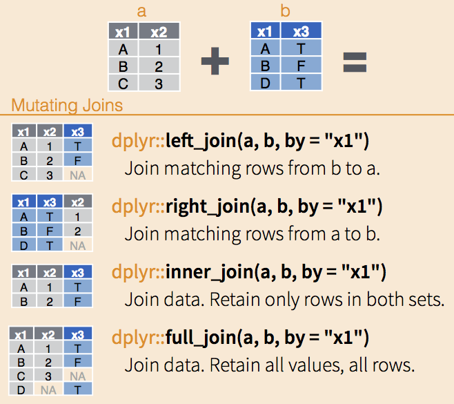
we can also join two or multiple data frames together.
- left_join()
  - keeps all the entries that are present in the left (first) table and excludes any that are only in the right table
- right_join()
  - keeps all the entries that are present in the right table and excludes any that are only in the left table.
- inner_join()
  - keeps only the entries that are present in both tables. inner_join is the only function that guarantees you won’t generate any missing entries.
- full_join()
  - keeps all of the entries in both tables, regardless of whether or not they appear in the other table.

2.3 Data visualization with ggplot2

> Data visualization is key to data story telling.

ggplot2 is a powerful package that enable publication ready plots
- easy customization (over SAS)
- clear syntax and lots of online template
- lots of extensions on style

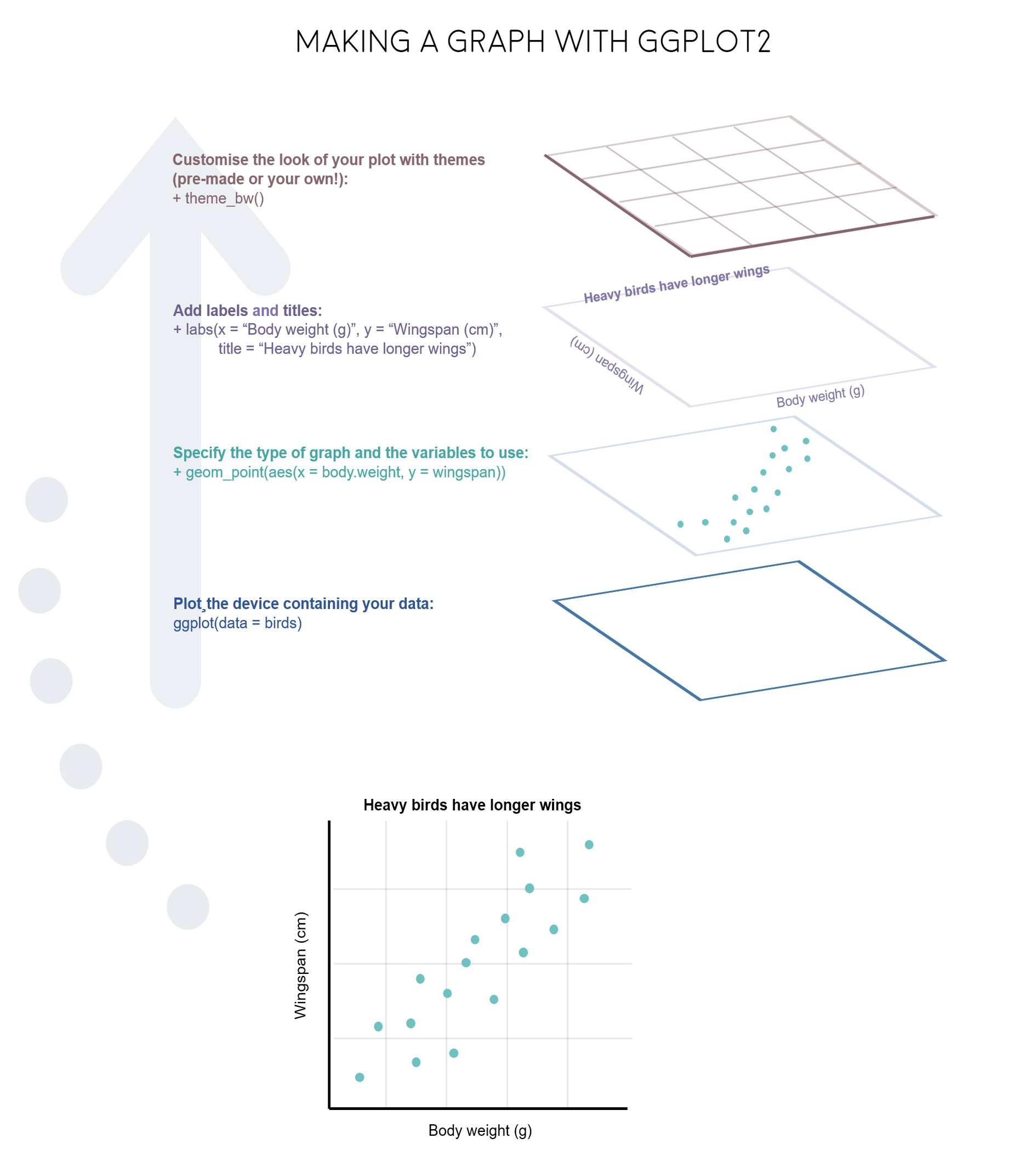
How ggplot2 works, https://codeahoy.com/learn/rtutorial/ch8/

ggplot components (from Wickham, 2009)

layer is a collection of geometric elements and statistical transformations.
aesthetic(aes) is “something you can see”.
- x, y: variable along the x and y axis
- colour: color of geoms according to data
- fill: the inside color of the geom
- group: what group a geom belongs to
- shape: the figure used to plot a point
- linetype: the type of line used (solid, dashed, etc)
- size: size scaling for an extra dimension
- alpha: the transparency of the geom
geometric elements (geoms), represent what you actually see in the plot: points, lines, polygons, etc.
- geom_area() draws an area plot
- geom_bar(stat="identity") draws a bar chart
- geom_line() draws a line
- geom_point() draws a scatterplot
- geom_rect(), draws rectangles
scales map values in the data space to values in the aesthetic space.
- This includes the use of colour, shape or size.
- Scales also draw the legend and axes
coordinate(coord), describes how data coordinates
- provides axes and gridlines to help read the graph.
facet specifies how to break up and display subsets of data as small multiples.
theme controls display style, like the font size and background colour.

Layers

ggplot(aes(x = decimal, y = average), data = co2)

Geometry

ggplot(aes(x = decimal, y = average), data = co2)+
  geom_point() +
  geom_line(color = "blue")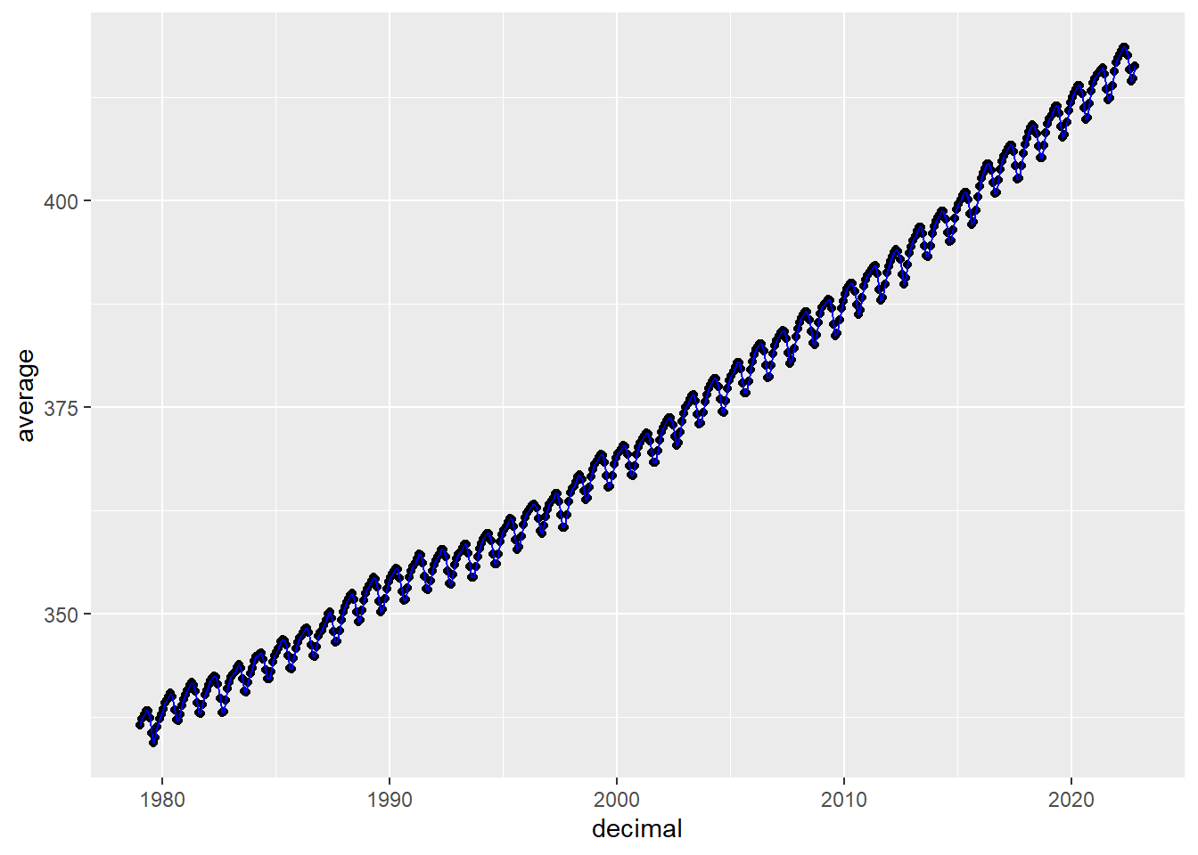

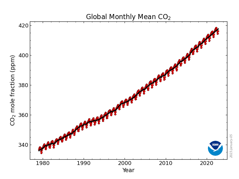
comparing to the plot provided on https://gml.noaa.gov/ccgg/trends/

Expand To Learn About various geoms

geom_abline: Reference lines: horizontal, vertical, and diagonal
geom_area: Ribbons and area plots
geom_bar: Bar charts
geom_boxplot: A box and whiskers plot
geom_contour: 2d contours of a 3d surface
geom_count: Count overlapping points
geom_crossbar: Vertical intervals: lines, crossbars & errorbars
geom_curve: Line segments and curves
geom_density: Smoothed density estimates
geom_dotplot: Dot plot
geom_errorbar: Vertical intervals: lines, crossbars & errorbars
geom_errorbarh: Horizontal error bars
geom_freqpoly: Histograms and frequency polygons
geom_hex: Hexagonal heatmap of 2d bin counts
geom_histogram: Histograms and frequency polygons
geom_hline: Reference lines: horizontal, vertical, and diagonal
geom_jitter: Jittered points
geom_label: Text
geom_line: Connect observations
geom_linerange: Vertical intervals: lines, crossbars & errorbars
geom_map: Polygons from a reference map
geom_path: Connect observations
geom_pointrange: Vertical intervals: lines, crossbars & errorbars
geom_polygon: Polygons
geom_qq: A quantile-quantile plot
geom_qq_line: A quantile-quantile plot
geom_quantile: Quantile regression
geom_raster: Rectangles
geom_ribbon: Ribbons and area plots
geom_rug: Rug plots in the margins
geom_segment: Line segments and curves
geom_smooth: Smoothed conditional means
geom_step: Connect observations
geom_text: Text
geom_tile: Rectangles
geom_violin: Violin plot
geom_vline: Reference lines: horizontal, vertical, and diagonal

labs, axis, facet, and theme

ggplot(aes(x = month, y = average), data = co2)+
  geom_point(alpha = 0.5) +  
  geom_line(color = "blue") +
  labs(
    x = 'Month',
    y = 'CO2 mole fraction (ppm)',
    title = 'Global Monthly Mean CO2'
  ) +
  scale_x_continuous(breaks = c(1,5,9,12)) +
  scale_y_continuous(breaks = seq(from=300,to=450,by=50)) +
  facet_wrap(vars(year)) +
  theme_bw()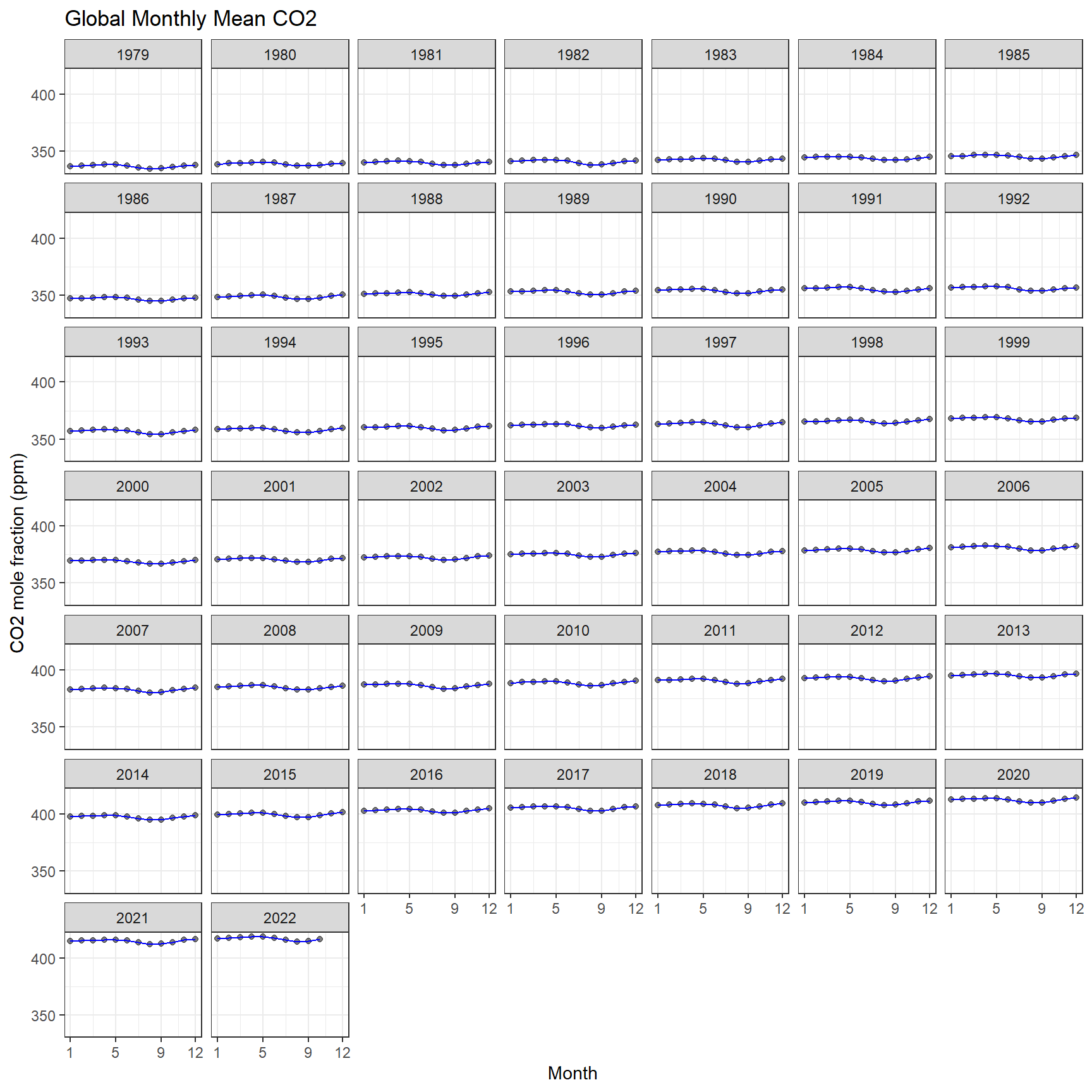

adding statistics

co2 %>%
  filter(year == 2021) %>%
  ggplot(aes(x = month, y = average))+
  geom_point() +
  geom_line(color="blue") +
  geom_smooth(formula = y ~ x, method = 'lm', color = "red") +
  geom_smooth(formula = y ~ splines::bs(x,3), method = 'lm', color = "orange") +
  scale_x_continuous(breaks = seq(1,12,1)) +
  labs(x = 'Month', y = 'CO2 mole fraction (ppm)', title = 'Global Monthly Mean CO2 in 2021')+ 
  theme_bw()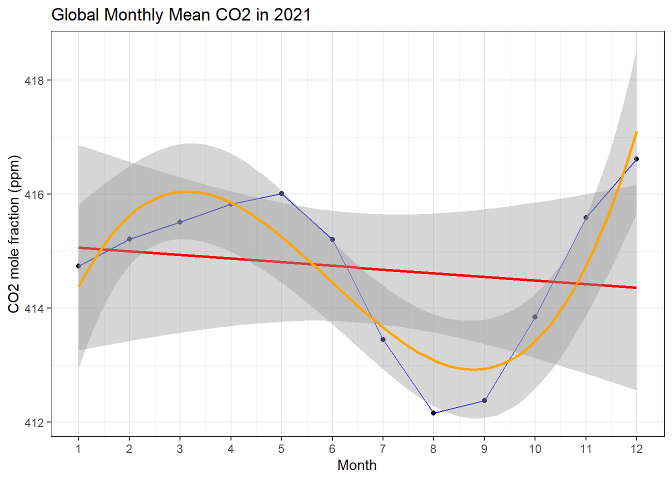

colours in R

require(RColorBrewer)

Loading required package: RColorBrewer

display.brewer.all()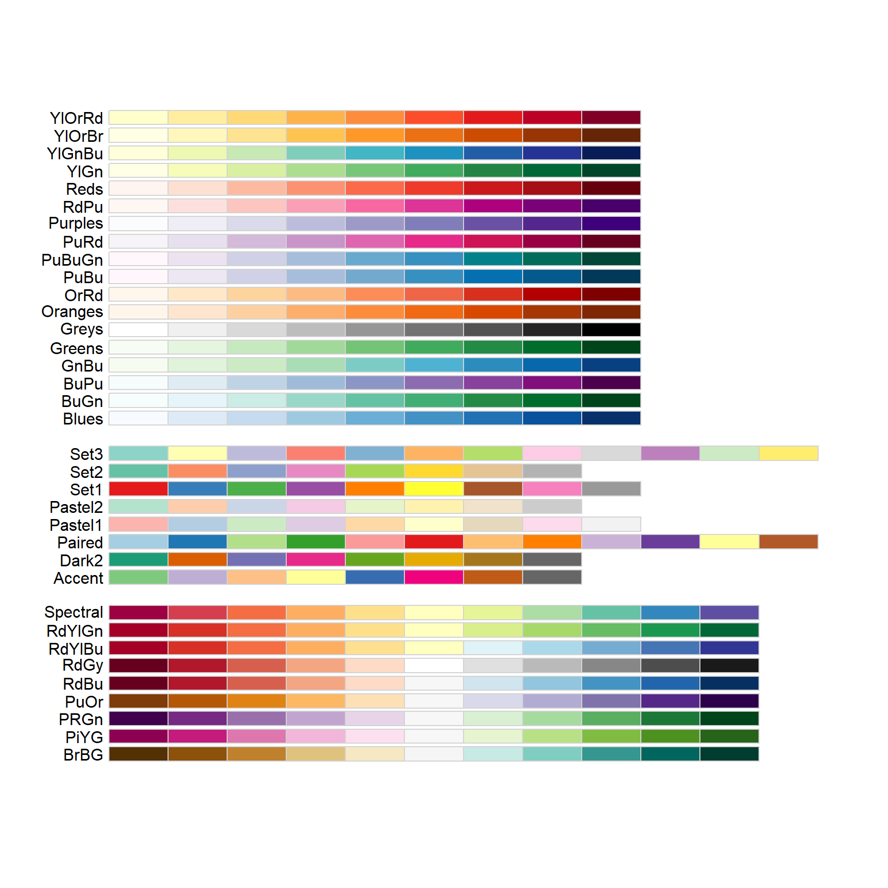

Other representative plots

Boxplot

Suppose we want to look at CO2 distribution by year

ggplot(data = co2, aes(x=year_group, y=average, fill=year_group)) + 
  geom_boxplot(alpha=0.3) +
  scale_fill_brewer(palette="Reds")+ 
  labs(x = 'Year Group', 
       y = 'CO2 mole fraction (ppm)', 
       title = 'Global Monthly Mean CO2 by Year Group',
       fill = 'Year group')+ 
  theme_bw()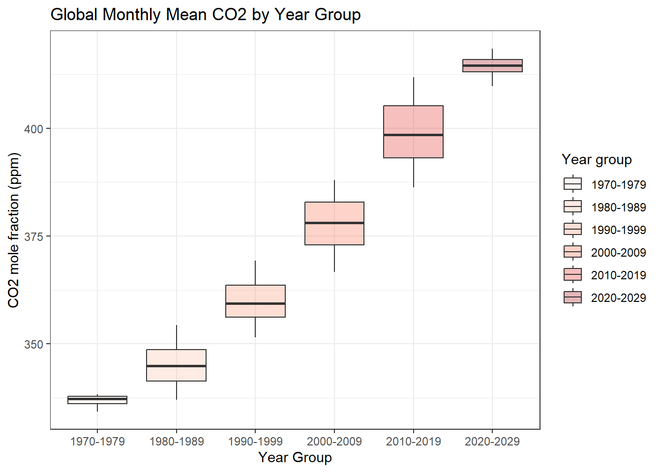

Heatmaps
we are interested to look at the pattern of CO2 concentration by year and month
three data dimensions: year, month, and value of co2

ggplot(data = co2, aes(y=factor(year), x=factor(month), fill=average)) + 
  geom_tile(colour = "white") +
  scale_x_discrete(position = "top") +
  scale_fill_distiller(palette = "Reds", direction = 1) +  
  labs(x = 'Month', 
       y = 'Year', 
       title = 'Global Monthly Mean CO2')+ 
  theme_bw()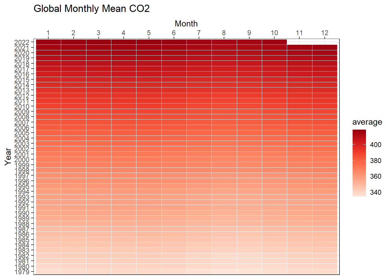

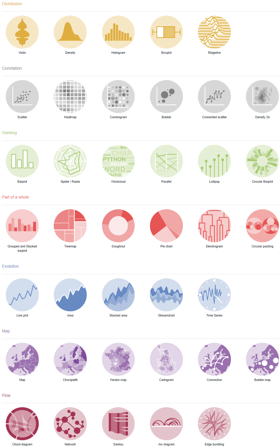
The R Graph Gallery, https://r-graph-gallery.com/index.html

Best reference for plotting with ggplot2 in R, https://r-graph-gallery.com/index.html