2. Using machine learning techniques for causal analysis

Author

Kuan Liu

Published

2024-10-12

Outlines

Propensity score methods machine learning techniques
- gradient boosting machines
- super learner
- Bayesian additive regression trees

Proposensity score analysis using machine learning technqiues

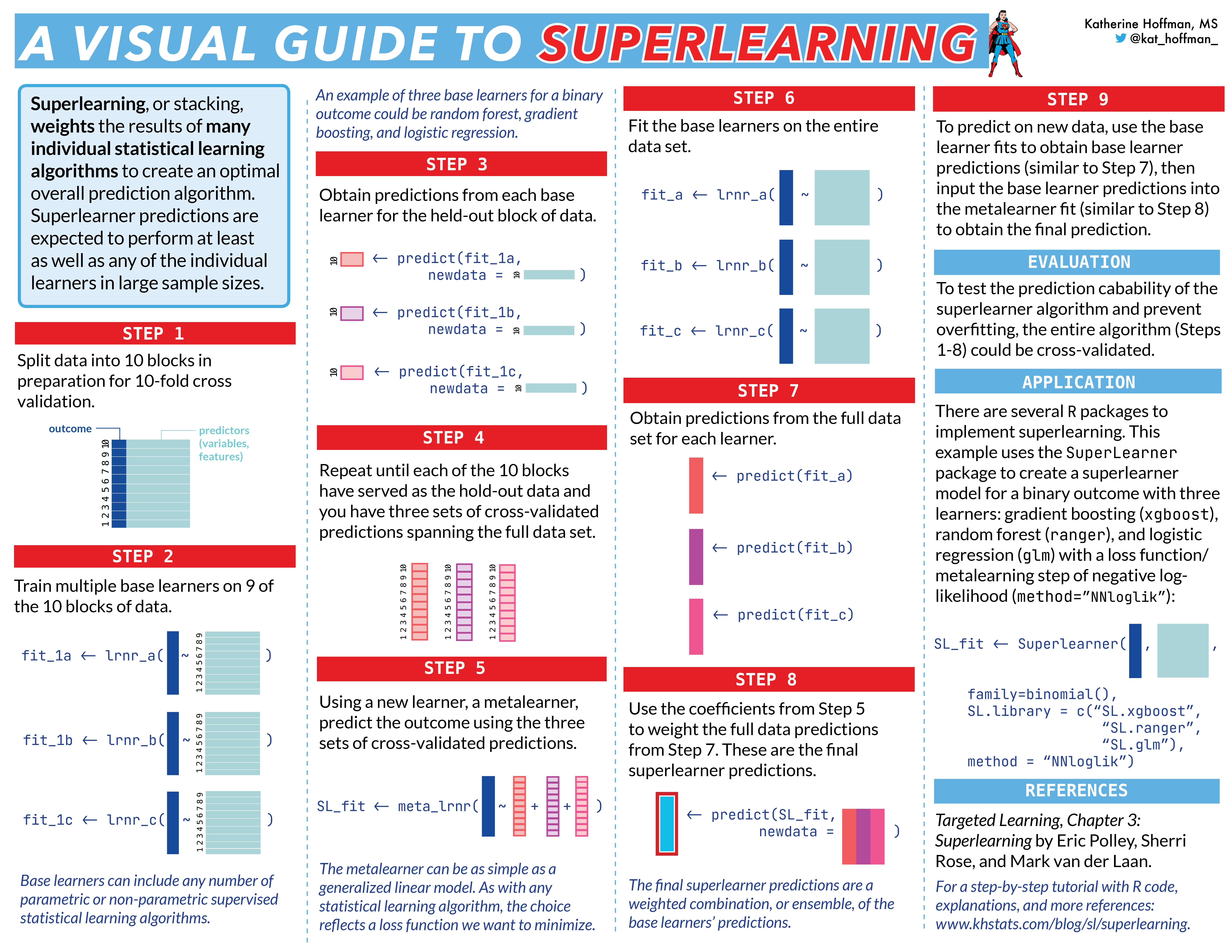
2.1 Super (Machine) Learning

Super learning can be used to obtain robust estimator. In a nut-shell it uses loss-function based ML tool and cross-validation to obtain the best prediction of model parameter of interest, based on a weighted average of a library of machine learning algorithms.
Guide to SuperLearner by Chris Kennedy at https://cran.r-project.org/web/packages/SuperLearner/vignettes/Guide-to-SuperLearner.html
New visual guide created by Katherine Hoffman

List of machine learning algorithms under SuperLearner R package

library(SuperLearner)
listWrappers()

 [1] "SL.bartMachine"      "SL.bayesglm"         "SL.biglasso"        
 [4] "SL.caret"            "SL.caret.rpart"      "SL.cforest"         
 [7] "SL.earth"            "SL.gam"              "SL.gbm"             
[10] "SL.glm"              "SL.glm.interaction"  "SL.glmnet"          
[13] "SL.ipredbagg"        "SL.kernelKnn"        "SL.knn"             
[16] "SL.ksvm"             "SL.lda"              "SL.leekasso"        
[19] "SL.lm"               "SL.loess"            "SL.logreg"          
[22] "SL.mean"             "SL.nnet"             "SL.nnls"            
[25] "SL.polymars"         "SL.qda"              "SL.randomForest"    
[28] "SL.ranger"           "SL.ridge"            "SL.rpart"           
[31] "SL.rpartPrune"       "SL.speedglm"         "SL.speedlm"         
[34] "SL.step"             "SL.step.forward"     "SL.step.interaction"
[37] "SL.stepAIC"          "SL.svm"              "SL.template"        
[40] "SL.xgboost"

[1] "All"
[1] "screen.corP"           "screen.corRank"        "screen.glmnet"        
[4] "screen.randomForest"   "screen.SIS"            "screen.template"      
[7] "screen.ttest"          "write.screen.template"

2.2 Using machine learning methods with PSA

We can use ML to model our propensity score model
The use of machine learning methods is more flexible than parametric methods (i.e., logistic regression)
- Not without a cost, usually the more flexible the methods are the more one is at risk of overfitting; Too much noise considered in the modelling often results in poor coverage probability.
- There is no one approach that out performs others, thus which approach to use should be evaluated case by case.
- ML is generally suggested for large enough cohort and for modelling large set of covariates.
- It’s always suggested to include results from conventional logistic regression approach as a sensitivity analysis in comparison of ML approaches.
Many approaches are included in the WeightIt package, https://ngreifer.github.io/WeightIt/reference/method_super.html
- “gbm”, Propensity score weighting using generalized boosted modeling (also known as gradient boosting machines)
- “super”, Propensity score weighting using SuperLearner
- “bart”, Propensity score weighting using Bayesian additive regression trees (BART)
  - Bayesian Additive Regression Trees (BART) is a sum-of-trees model for approximating an unknown function. To avoid overfitting (of decision tree), BART uses a regularization prior that forces each tree to be able to explain only a limited subset of the relationships between the covariates and the predictor variable.

Setting up data and PS model formula

require(tidyverse)
require(WeightIt)
data2<-readRDS("data/data2")
covariates <- select(data2, -c(id, A, Y))
baselines <- colnames(covariates)

ps.formula <- as.formula(paste("A~", 
                paste(baselines, collapse = "+")))

2.2.1 PS model with gradient boosting

computationally more demanding and it might take several minutes to run.

IPTW_gbm <- weightit(ps.formula,
                 data = data2,
                 method = "gbm",
                 stabilize = TRUE)
# saving the model output as a R object to avoid rerunning the same model;
saveRDS(IPTW_gbm, file = "data/IPTW_gbm")

# reading saved model output;
require(sjPlot)
IPTW_gbm <- readRDS(file = "data/IPTW_gbm")
summary(IPTW_gbm)

                  Summary of weights

- Weight ranges:

           Min                                   Max
treated 0.3874 |---------------------------| 10.9875
control 0.6227  |------------|                5.6764

- Units with the 5 most extreme weights by group:
                                            
           5525   3148   4890   1825    5131
 treated 4.0556 4.6873 5.1931 5.3152 10.9875
            497   2046   3830   1602    1000
 control 4.6689 4.8977  4.929 4.9313  5.6764

- Weight statistics:

        Coef of Var   MAD Entropy # Zeros
treated       0.663 0.397   0.143       0
control       0.426 0.262   0.067       0

- Effective Sample Sizes:

           Control Treated
Unweighted 3551.   2184.  
Weighted   3006.24 1517.47

fit2_gbm <- glm_weightit(Y ~ A, 
            family = "binomial",
            weightit = IPTW_gbm,
            data = data2)
tab_model(fit2_gbm)

	Y
Predictors	Odds Ratios	CI	p
(Intercept)	0.46	0.42 – 0.49	<0.001
A	1.27	1.11 – 1.44	<0.001
Observations	5735
R² Tjur	0.004

2.2.2 PS model with Super Learner

IPTW_SL <- weightit(ps.formula,
                 data = data2,
                 method = "super",
                 SL.library=c("SL.randomForest", "SL.glmnet", "SL.nnet"), 
                 stabilize = TRUE)
# saving the model output as a R object to avoid rerunning the same model;
saveRDS(IPTW_SL, file = "data/IPTW_SL")

# reading saved model output;
IPTW_SL <- readRDS(file = "data/IPTW_SL")
summary(IPTW_SL)

                  Summary of weights

- Weight ranges:

           Min                                  Max
treated 0.4008 |-----------------|           1.0346
control 0.6254        |--------------------| 1.4140

- Units with the 5 most extreme weights by group:
                                           
            742   5131   3508   1825   4890
 treated 0.9223 0.9489  0.968 0.9808 1.0346
           3391   3216   2174   2986    505
 control 1.3373 1.3461 1.3533 1.3627  1.414

- Weight statistics:

        Coef of Var   MAD Entropy # Zeros
treated       0.184 0.147   0.016       0
control       0.159 0.125   0.012       0

- Effective Sample Sizes:

           Control Treated
Unweighted 3551.    2184. 
Weighted   3463.76  2112.6

fit2_SL <- glm_weightit(Y ~ A, 
            family = "binomial",
            weightit = IPTW_SL,
            data = data2)
tab_model(fit2_SL)

	Y
Predictors	Odds Ratios	CI	p
(Intercept)	0.45	0.42 – 0.48	<0.001
A	1.35	1.21 – 1.51	<0.001
Observations	5735
R² Tjur	0.005

2.2.3 PS model with Bayesian additive regression trees

A much faster algorithm comparing to gbm and SL.

IPTW_bart <- weightit(ps.formula,
                 data = data2,
                 method = "bart",
                 stabilize = TRUE)
# saving the model output as a R object to avoid rerunning the same model;
saveRDS(IPTW_bart, file = "data/IPTW_bart")

# reading saved model output;
IPTW_bart <- readRDS(file = "data/IPTW_bart")
summary(IPTW_bart)

                  Summary of weights

- Weight ranges:

           Min                                   Max
treated 0.3861 |---------------------------| 13.8560
control 0.6211 |------------------|           9.8333

- Units with the 5 most extreme weights by group:
                                             
           3148   4119    1825    5131   4890
 treated 8.7361 9.5095 11.8258 12.7766 13.856
             84   1810    3839    1000    505
 control 6.7109 6.7279  7.9066  7.9218 9.8333

- Weight statistics:

        Coef of Var   MAD Entropy # Zeros
treated       0.926 0.471   0.226       0
control       0.544 0.308   0.096       0

- Effective Sample Sizes:

           Control Treated
Unweighted 3551.   2184.  
Weighted   2740.56 1175.59

fit2_bart <- glm_weightit(Y ~ A, 
            family = "binomial",
            weightit = IPTW_bart,
            data = data2)
tab_model(fit2_bart)

	Y
Predictors	Odds Ratios	CI	p
(Intercept)	0.45	0.42 – 0.49	<0.001
A	1.30	1.13 – 1.50	<0.001
Observations	5735
R² Tjur	0.005

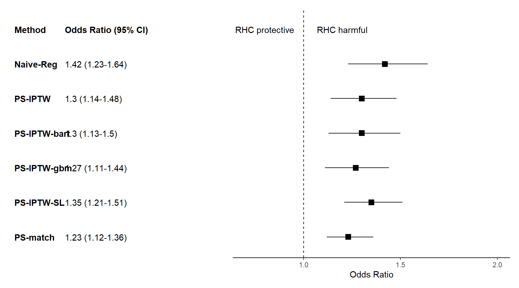
Comparing the three approaches given the rhc data, it appears that SuperLearner returns good stable weights (no visible extreme weights). This indicates a great fit of the PS model.

Similar as before, we can check for PS distribution and balancing. Additionally, we can perform subgroup and sensitivity analysis as mentioned before.

Forest plot to display results from different approaches

code modified from https://www.khstats.com/blog/forest-plots/ by Katherine Hoffman

plotdata <- data.frame(
  method = c("Naive-Reg","PS-match", "PS-IPTW", "PS-IPTW-gbm", "PS-IPTW-SL", "PS-IPTW-bart"),  
  est.OR = c(1.42, 1.23, 1.30, 1.27, 1.35, 1.30),
  conf.low = c(1.23, 1.12, 1.14, 1.11, 1.21, 1.13),
  conf.high = c(1.64, 1.36, 1.48, 1.44, 1.51, 1.50))

p <- 
  plotdata |>
  ggplot(aes(y = fct_rev(method))) + 
  theme_classic() +
  geom_point(aes(x=est.OR), shape=15, size=3) +
  geom_linerange(aes(xmin=conf.low, xmax=conf.high)) +
  geom_vline(xintercept = 1, linetype="dashed") +
  labs(x="Odds Ratio", y="") +
  coord_cartesian(ylim=c(1,7), xlim=c(0.7, 2)) +
  annotate("text", x = 0.8, y = 7, label = "RHC protective") +
  annotate("text", x = 1.2, y = 7, label = "RHC harmful") + 
  theme(axis.line.y = element_blank(),
        axis.ticks.y= element_blank(),
        axis.text.y= element_blank(),
        axis.title.y= element_blank())


plotdata_OR <- plotdata |>
  # round estimates and 95% CIs to 2 decimal places for journal specifications
  mutate(estimate_label = paste0(est.OR, " (", conf.low, "-", conf.high, ")"))  |>
  # add a row of data to be shown on the forest plot as column names;
  bind_rows(
    data.frame(
      method = "Method",
      estimate_label = "Odds Ratio (95% CI)"
    )
  ) |>
  mutate(method = fct_rev(fct_relevel(method, "Method")))

p_left <-
  plotdata_OR  |>
  ggplot(aes(y = method)) +
  geom_text(aes(x = 0, label = method), hjust = 0, fontface = "bold")+
  geom_text(
    aes(x = 1, label = estimate_label),
    hjust = 0,
    fontface = ifelse(plotdata_OR$estimate_label == "Odds Ratio (95% CI)", "bold", "plain")
  )+
  theme_void() +
  coord_cartesian(xlim = c(0, 4))

library(patchwork)
layout <- c(
  area(t = 0, l = 0, b = 14, r = 4), # left plot, starts at the top of the page (0) and goes 14 units down and 4 units to the right;
  area(t = 1, l = 5, b = 14, r = 9) # middle plot starts a little lower (t=1) because there's no title. starts 1 unit right of the left plot (l=5, whereas left plot is r=4);
)
# final plot arrangement
p_left + p +plot_layout(design = layout)