Session 6 Bayesian Regression I

• Learn how to fit linear regression model with brms
• Understand how to interpret and report regression posterior results
• Learn how to fit clustered data with brms
• Learn how to conduct model diagnostics, model comparison, and variable selection

What is regression? (McElreath 2018)

• using one or more predictor variables to model the distribution of one or more outcome variables

• For a continuous outcome, we typically fit a linear regression model.

  • Of course the relationship between outcome and predictors can be non-linear, in this case, we would consider fitting polynomial regression models or splines.

• For a categorical outcome, we will fit a generalized linear regression. We will cover this topic in future sessions.

• For a repeatedly measured outcome, we can fit a linear mixed-effect model (continuous outcome) or a generalized linear mixed-effect model (categorical outcome).

6.1 Normal Models and Linear Regression

Conditional normal model

• Given its mean and variance, an observation has a normal distribution

\[ Y_i \mid \mu_i, \sigma^2_i \sim N( \mu_i, \sigma^2_i) \]

• This is equivalent to the following statements

\[ Y_i = \mu_i + e_i , \ e_i \sim N(0, \sigma^2)\]

• We do not assume the collection of \(Y_i, i=1, \ldots, n\) have a normal distribution

• Instead we assume the error term is normally distributed - a lesser assumption!

• In case of multiple predictors, \(\mu_i\) becomes a weighted average of the \(\beta_j\) values, the regression coefficient with \(x_{ij}\) denoting the predictors. For example, for two covariates we have

\[ E(y_i) = \mu_i = \beta_0 + \beta_1 x_{i1} + \beta_2 x_{i2} \]

• A polynomial regression model of 2 degrees on \(x_{i1}\)

\[ \mu_i = \beta_0 + \beta_1 x_{i1} + \beta_2 x_{i2} + \beta_3 x_{i1}^2 \]

• Assumptions of linear regression models
  1. Independent observations
  2. Linear relationship We can check this assumption by examining marginal plots comparing the model predicted relationship between outcome and each continuous predictor and by examining the residual plot.
  3. Normality of the residuals
  4. Homoscedasticity Homoscedasticity in a model means that the residual is constant along the values of the dependent variable.
  5. Multicollinearity Multicollinearity is the phenomenon when a number of the explanatory variables are strongly correlated.
  6. Correctly specified regression model This means that all relevant predictors for the response variable have been included in the model. This is often difficult to verify, but we can use posterior predictive distribution to check for regression fit.

6.1.1 One-sample and two-sample normal regression

1. One-sample

• If all observations have the same mean and variance, the likelihood is

\[ Y_i \mid \mu, \sigma^2 \sim N(\mu, \sigma^2)\]

• Good candidate priors for \(mu\) and \(\sigma\) are
  • \(\mu \sim N(\text{sample mean}, \text{sample sd})\) or Student-T distributions (to handle heavy tails)
  • \(\sigma \sim \text{half-t}(mean = 0, sd = \text{sample sd}, df = 3)\)

Modelling height - Textbook example on the Howell data

Suppose we want to fit a one-sample model on height using a dataset of anthropological measurements on a foraging people taken in the 1960s.

• First let’s examine the summary statistics of variable height

dat <- read.table("data/Howell.txt",header=T, sep=";")

dat %>% tbl_summary(
    statistic = list(all_continuous() ~ "{mean} ({sd})",
                     all_categorical() ~ "{n} / {N} ({p}%)"),
    digits = all_continuous() ~ 2)

Characteristic	N = 5441
height	138.26 (27.60)
weight	35.61 (14.72)
age	29.34 (20.75)
male	257 / 544 (47%)
1 Mean (SD); n / N (%)

dat %>% pivot_longer(everything()) %>% 
  mutate(name = factor(name, levels = c("height", "weight", "age", "male"))) %>% ggplot(aes(x = value)) +
  geom_histogram(bins = 10,fill="#008BB0",colour="#002A5C") +
  facet_wrap(~name, scales = "free", ncol = 1) +
  theme_bw()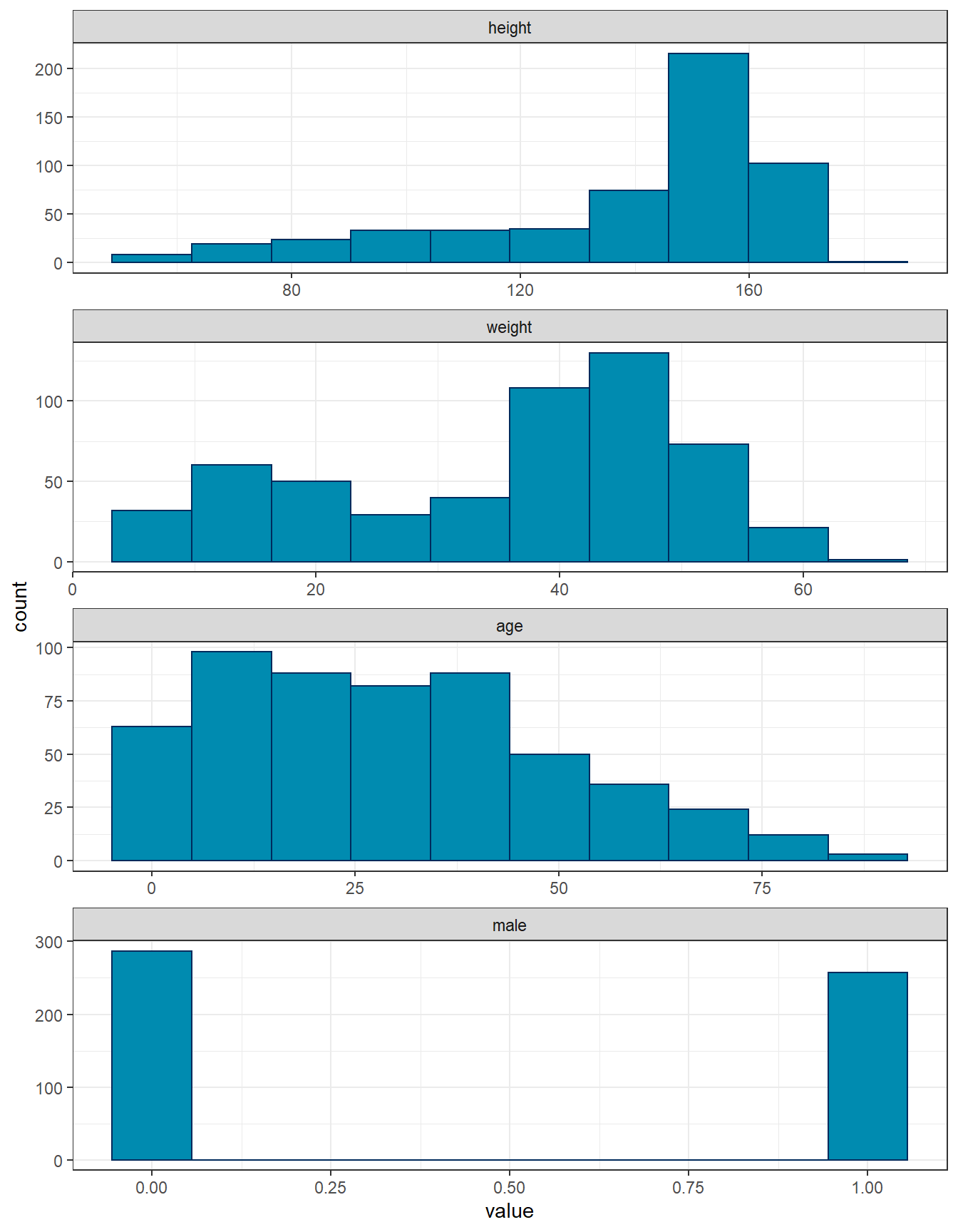

• We specify our model with the following priors \[ heights_i \sim N (\mu, \sigma)\] \[\mu \sim N(138, 28)\] \[\sigma \sim \text{half-t}(0, 28, df = 3)\]

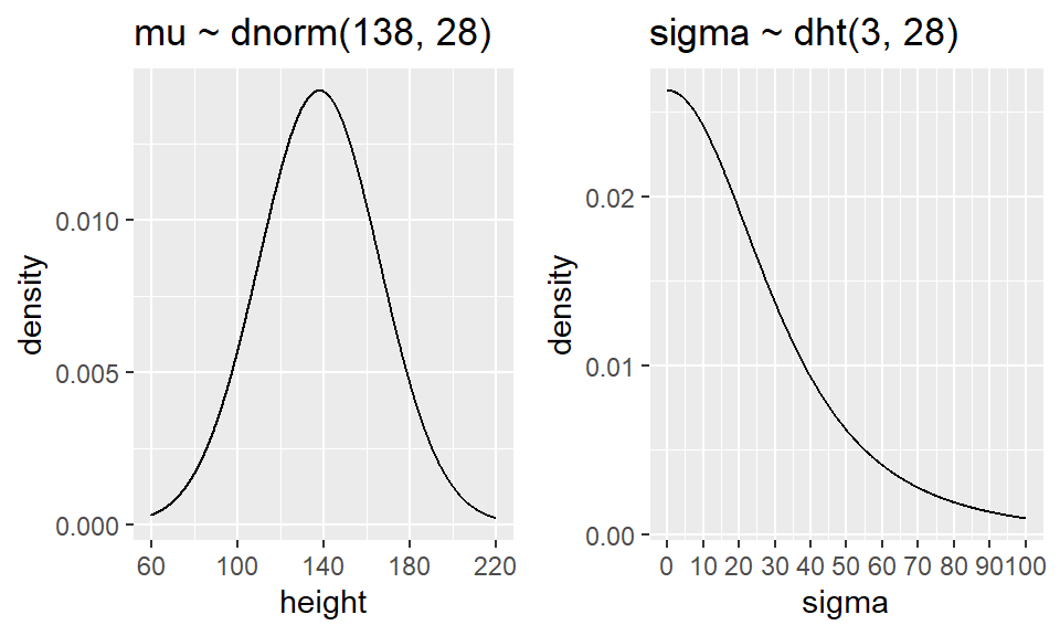
Figure 6.1: Prior distributions

• we now fit this model in brms

fit0 <- brm(data = dat,
             family = gaussian,
             height ~ 1, 
             prior = c(prior(normal(138, 28), class = Intercept),
                       prior(student_t(3, 0, 28), class = sigma)),
             iter = 10000, 
             warmup = 5000, 
             chains = 4, 
             cores = 4, #instructions on MCMC
             seed = 123, # random number seed to make results reproducible
             silent = 2,
             refresh = 0)

# saveRDS(fit0, "data/chap7_onesample_example")

• Summarizing posterior results

##  Family: gaussian 
##   Links: mu = identity; sigma = identity 
## Formula: height ~ 1 
##    Data: dat (Number of observations: 544) 
##   Draws: 4 chains, each with iter = 10000; warmup = 5000; thin = 1;
##          total post-warmup draws = 20000
## 
## Population-Level Effects: 
##           Estimate Est.Error l-95% CI u-95% CI Rhat Bulk_ESS Tail_ESS
## Intercept   138.25      1.18   135.94   140.58 1.00    18944    14350
## 
## Family Specific Parameters: 
##       Estimate Est.Error l-95% CI u-95% CI Rhat Bulk_ESS Tail_ESS
## sigma    27.64      0.84    26.06    29.35 1.00    18557    13633
## 
## Draws were sampled using sampling(NUTS). For each parameter, Bulk_ESS
## and Tail_ESS are effective sample size measures, and Rhat is the potential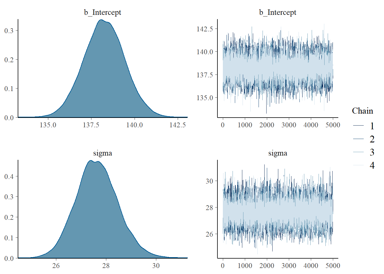
## scale reduction factor on split chains (at convergence, Rhat = 1).

• Geweke index and R-hat (Geweke et al. 1991) to check for MCMC convergence

# modelposterior <- as.mcmc(fit0)
# geweke.plot(modelposterior)
modelposterior <- posterior_samples(fit0)
geweke.diag(modelposterior)

## 
## Fraction in 1st window = 0.1
## Fraction in 2nd window = 0.5 
## 
## b_Intercept       sigma        lp__ 
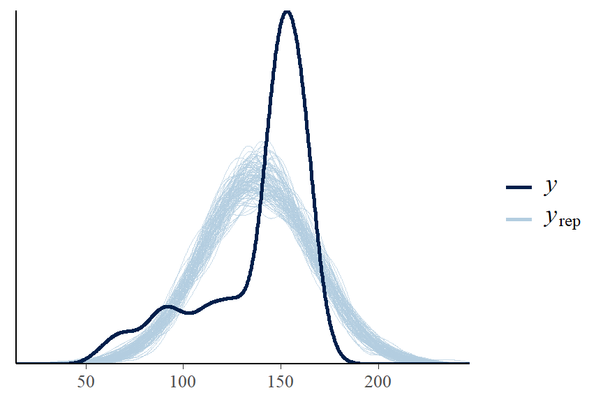
##      0.4570      0.2874      0.9759

• Posterior predictive graphic check for model fit
  • we can see here there is some skewness not captured in the model, this model is not a good fit to the data.
  • we will revisit the height model in the linear regression section where we add covariates to the model to improve the fit.

What is the posterior evidence that mean height is greater than 140cm?

hypothesis(fit0, 'Intercept > 140' , alpha = 0.025)

# proportion of posterior samples on the mean (intercept) 
# with value > 140, combining 4 chains;
modelposterior2<- posterior_samples(fit0)
sum(modelposterior2[,1]>140)/length(modelposterior2[,1])

2. Two-sample

• Simple extension of the one-sample problem
• Observations within the each group have the same mean and variance, yielding the following likelihood \[ Y_{ji} \mid \mu_j, \sigma^2_j \sim N(\mu_j, \sigma^2_j)\]
• Similar candidate prior as in one-sample model
  • using normal or student-t dist and observed summary statistics
  • within-group variance should be smaller than the variance when we ignore groups
• We can assume equal variance \(\sigma_1^2 = \sigma_2^2\) or allow them to be estimated seperately
• These two approaches are analogous to the equal-variance and unequal-variance t-tests
• In brms, this is easy to specify

Modelling hours of sleep comparing between two drugs

• Data which show the effect of two medication (within-patient increase in hours of sleep) on groups consisting of 10 patients each.

• Source: Student (1908) The probable error of a mean. (Student 1908)

• First examine the summary statistics by group

sleep <- data.frame(extra = c(0.7, -1.6, -0.2, -1.2, -0.1, 3.4, 3.7, 0.8, 0, 2, 1.9, 0.8, 1.1, 0.1, -0.1, 4.4, 5.5, 1.6, 4.6, 3.4), 
                group = c(1, 1, 1, 1, 1, 1, 1, 1, 1, 1, 2, 2, 2, 2, 2, 2, 2, 2, 2, 2))

sleep %>% 
  mutate(group = recode_factor(group,  '1'="Drug A", '2'="Drug B")) %>%
  tbl_summary(
    by = group,
    statistic = all_continuous() ~ "{mean} ({sd})",
    digits = all_continuous() ~ 2) %>%
  add_overall()

Characteristic	Overall, N = 201	Drug A, N = 101	Drug B, N = 101
extra	1.54 (2.02)	0.75 (1.79)	2.33 (2.00)
1 Mean (SD)

• Fitting two-sample model in brms using default brms prior
  • student_t(3, 1, 2.5) for mean (same for each group)
  • student_t(3, 0, 2.5) for sigma (same for each group for unequal variance model)

fit_eq <- brm(data = sleep,
             family = gaussian,
             extra ~ group, #mean depends on group and one sigma
             prior = c(prior(normal(0, 10), class = Intercept),
                       prior(normal(0,10), class = b),
                       prior(student_t(3, 0, 2), class = sigma)),
             iter = 10000, 
             warmup = 5000, 
             chains = 4, 
             cores = 4, #instructions on MCMC
             seed = 123, # random number seed to make results reproducible
             silent = 2,
             refresh = 0)

prior_summary(fit_eq)

fit_uneq <- brm(data = sleep,
             family = gaussian,
             bf(extra ~ group, #mean depends on group
             sigma ~ group), #sigma differ by group
             prior = c(prior(normal(0, 10), class = Intercept), #prior for intercept of the extra ~ group model;
                       prior(normal(0, 10), class = b), #prior for coefficients of the extra ~ group model;
                       prior(student_t(3, 0, 2), class = Intercept, dpar = "sigma"), #prior for intercept of the sigma ~ group model;
                       prior(student_t(3, 0, 2), class = b, dpar = "sigma")), #prior for coefficients of the sigma ~ group model;
             iter = 10000, 
             warmup = 5000, 
             chains = 4, 
             cores = 4, #instructions on MCMC
             seed = 123, # random number seed to make results reproducible
             silent = 2,
             refresh = 0)

prior_summary(fit_uneq)

# saveRDS(fit_eq, "data/chap7_twosample_eq")
# saveRDS(fit_uneq, "data/chap7_twosample_uneq")

• Summarizing posterior results from equal variance model

##  Family: gaussian 
##   Links: mu = identity; sigma = identity 
## Formula: extra ~ group 
##    Data: sleep (Number of observations: 20) 
##   Draws: 4 chains, each with iter = 10000; warmup = 5000; thin = 1;
##          total post-warmup draws = 20000
## 
## Population-Level Effects: 
##           Estimate Est.Error l-95% CI u-95% CI Rhat Bulk_ESS Tail_ESS
## Intercept     0.73      0.63    -0.55     1.98 1.00    16492    13222
## group2        1.57      0.91    -0.22     3.38 1.00    16232    12475
## 
## Family Specific Parameters: 
##       Estimate Est.Error l-95% CI u-95% CI Rhat Bulk_ESS Tail_ESS
## sigma     2.00      0.35     1.44     2.79 1.00    13907    12976
## 
## Draws were sampled using sampling(NUTS). For each parameter, Bulk_ESS
## and Tail_ESS are effective sample size measures, and Rhat is the potential
## scale reduction factor on split chains (at convergence, Rhat = 1).

• Question: What is the probability that there is more increase in sleep with drug A? (under equal-variance model)

samples <- posterior_samples(fit_eq)
difference <- samples[,"b_group2"]
#summarize the difference
c(Prob = mean(difference > 0), Mean = mean(difference), lowCrI = quantile(difference, 0.025), highCrI = quantile(difference, 1-0.025))

##          Prob          Mean   lowCrI.2.5% highCrI.97.5% 
##     0.9591500     1.5713935    -0.2217899     3.3785453

#we can also use hypothesis function to evaluate this
hypothesis(fit_eq, "group2 > 0", alpha = 0.025)

## Hypothesis Tests for class b:
##     Hypothesis Estimate Est.Error CI.Lower CI.Upper Evid.Ratio Post.Prob Star
## 1 (group2) > 0     1.57      0.91    -0.22     3.38      23.48      0.96     
## ---
## 'CI': 95%-CI for one-sided and 97.5%-CI for two-sided hypotheses.
## '*': For one-sided hypotheses, the posterior probability exceeds 97.5%;
## for two-sided hypotheses, the value tested against lies outside the 97.5%-CI.
## Posterior probabilities of point hypotheses assume equal prior probabilities.

• Summarizing posterior results from unequal variance model and evaluate the same hypothesis

fit_uneq <- readRDS("data/chap7_twosample_uneq")
summary(fit_uneq)

##  Family: gaussian 
##   Links: mu = identity; sigma = log 
## Formula: extra ~ group 
##          sigma ~ group
##    Data: sleep (Number of observations: 20) 
##   Draws: 4 chains, each with iter = 10000; warmup = 5000; thin = 1;
##          total post-warmup draws = 20000
## 
## Population-Level Effects: 
##                 Estimate Est.Error l-95% CI u-95% CI Rhat Bulk_ESS Tail_ESS
## Intercept           0.73      0.63    -0.54     1.97 1.00    15554    10549
## sigma_Intercept     0.63      0.25     0.20     1.17 1.00    15707    11003
## group2              1.57      0.94    -0.27     3.47 1.00    15377    12395
## sigma_group2        0.11      0.35    -0.57     0.80 1.00    14749    11864
## 
## Draws were sampled using sampling(NUTS). For each parameter, Bulk_ESS
## and Tail_ESS are effective sample size measures, and Rhat is the potential
## scale reduction factor on split chains (at convergence, Rhat = 1).

hypothesis(fit_uneq, "group2 > 0", alpha = 0.025)

## Hypothesis Tests for class b:
##     Hypothesis Estimate Est.Error CI.Lower CI.Upper Evid.Ratio Post.Prob Star
## 1 (group2) > 0     1.57      0.94    -0.27     3.47         21      0.95     
## ---
## 'CI': 95%-CI for one-sided and 97.5%-CI for two-sided hypotheses.
## '*': For one-sided hypotheses, the posterior probability exceeds 97.5%;
## for two-sided hypotheses, the value tested against lies outside the 97.5%-CI.
## Posterior probabilities of point hypotheses assume equal prior probabilities.

How to determine equal variance or not?

• Approach 1, visually examine the conditional mean by group.
• Approach 2, comparing models using information criteria (WAIC) or leave-one-out cross validation (LOO) (Vehtari, Gelman, and Gabry 2017)
• Both approaches confirm the equal variance model is the best model!

plot(conditional_effects(fit_uneq), points = TRUE)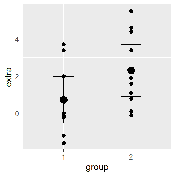

waic1 <- waic(fit_eq)
waic2 <- waic(fit_uneq)
compare_ic(waic1, waic2) #equal var best model;

##                    WAIC   SE
## fit_eq            85.98 4.25
## fit_uneq          87.57 4.54
## fit_eq - fit_uneq -1.59 0.60

loo1 <- loo(fit_eq)
loo2 <- loo(fit_uneq)
loo_compare(loo1, loo2) #equal var best model;

##          elpd_diff se_diff
## fit_eq    0.0       0.0   
## fit_uneq -0.9       0.3

6.1.2 Linear regression

• The two-sample model is a special case of regression

\[\mu_i = \beta_0 + \beta_1 x_i\]

• Where \(x_i = 0\) for group 1 and \(x_i = 1\) for group 2
  • For group 1, \(\mu_i = \beta_0\), the intercept
  • For group 2, \(\mu_i = \beta_0 + \beta_1\)
• brms takes care of creating dummy variables!
• but be aware of what the reference group is and what the coefficients mean
• levels will be by default in alphabetical order - use the factor() statement to make a variable with the desired order

Try fitting the two-sample sleep data without the intercept

fit_eq2 <- brm(data = sleep,
             family = gaussian,
             extra ~ -1 + group, #mean depends on group and one sigma
             iter = 10000, 
             warmup = 5000, 
             chains = 4, 
             cores = 4, #instructions on MCMC
             seed = 123, # random number seed to make results reproducible
             silent = 2,
             refresh = 0)
summary(fit_eq2)

• In general, for a regression model

\[ y_i \mid \mu_i, \sigma^2_i \sim N(\mu_i, \sigma^2_i)\] \[ \mu_i = \beta_0 + \beta_1 x_{i1} + \ldots + \beta_p x_{ip}\] - where the \(x_{ij}\) can be continuous variables or “dummy” variables - the usual assumption on the variance is \(\sigma_i^2 = \sigma^2\) for all subjects (Homoscedasticity - equal variance assumption) - We can seen that is technically easier to relax this assumption in a Bayesian model! (two-sample unequal variance example)

• Predictions
  • We can get the predictions fro the mean value at a given value of the predictors. For example, in simple linear regression model we have
  \[E(Y\mid X=x) = \beta_0 + \beta_1 x\]
  • but recall that both \(\beta_0\) and \(\beta_1\) have posterior distributions
  • For each posterior draws of \((\beta_0, \beta_1)^s, s= 1, \ldots, S\), we have a different predicted mean
  \[E(Y\mid X=x, S=s) = \beta_0^s + \beta_1^s x\]
  • The set of values of these predictions across all sampled values give the posterior for the predicted mean

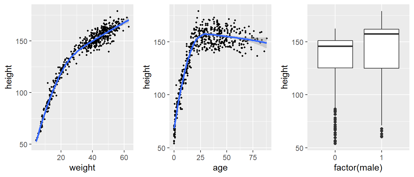
Modelling height - Howell data revisit

• Let’s descriptively examine the height distribution by weight, age, and sex
  • We can see that the relationship between age and height is not linear
  • we consider the following model
  \[heights_i \sim N(\mu_i, \sigma)\] \[\mu_i = \beta_0 + \beta_1 \ weight_i + \beta_2 \ age_i + \beta_3 \ age_i^2 +\beta_4 \ \text{I(sex=male)}\]

• we consider the following prior distributions (diffuse normal on regression parameter and exponential distribution for \(\sigma\)) \[\beta_0 \sim N(0, 100) \] \[\beta_1 \sim N(0, 10) \] \[\beta_2 \sim N(0, 10) \] \[\beta_3 \sim N(0, 10) \] \[\beta_4 \sim N(0, 10) \] \[ \sigma \sim Gamma(1, 0.01) \]

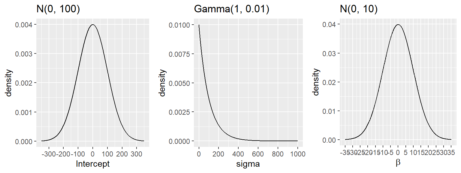
Figure 6.2: Prior distributions

• we now fit this model in brms

dat <- dat %>% 
  mutate(male = factor(male, labels = c("female", "male")))

fit1 <- brm(data = dat,
             family = gaussian,
             height ~ weight + age + I(age^2) + male,
             prior = c(prior(normal(0, 100), class = Intercept),
                       # set for all "b" coefficients
                       prior(normal(0, 10), class = b),
                       prior(gamma(1, 0.01), class = sigma)),
             iter = 20000,
             warmup = 18000,
             chains = 4,
             cores = 4, #instructions on MCMC
             seed = 123, # random number seed to make results reproducible
             silent = 2,
             refresh = 0)

# saveRDS(fit1, "data/chap7_reg_example")

• Summarizing posterior results

##  Family: gaussian 
##   Links: mu = identity; sigma = identity 
## Formula: height ~ weight + age + I(age^2) + male 
##    Data: dat (Number of observations: 544) 
##   Draws: 4 chains, each with iter = 20000; warmup = 18000; thin = 1;
##          total post-warmup draws = 8000
## 
## Population-Level Effects: 
##           Estimate Est.Error l-95% CI u-95% CI Rhat Bulk_ESS Tail_ESS
## Intercept    75.53      1.01    73.52    77.50 1.00     8716     6882
## weight        1.26      0.06     1.15     1.37 1.00     3406     4486
## age           1.06      0.11     0.84     1.29 1.00     3169     4137
## IageE2       -0.01      0.00    -0.01    -0.01 1.00     3297     4224
## malemale      1.86      0.80     0.33     3.41 1.00     5375     4740
## 
## Family Specific Parameters: 
##       Estimate Est.Error l-95% CI u-95% CI Rhat Bulk_ESS Tail_ESS
## sigma     8.70      0.27     8.20     9.23 1.00     6501     5373
## 
## Draws were sampled using sampling(NUTS). For each parameter, Bulk_ESS
## and Tail_ESS are effective sample size measures, and Rhat is the potential
## scale reduction factor on split chains (at convergence, Rhat = 1).

• Using the posterior mean, we have the following regression line

\[\hat{height}_i = 75.53 + 1.26 \ weight_i + 1.06 \ age_i -0.01 \ age_i^2 + 1.86 \ \text{I(sex=male)}\]

• Comparing between male and female of the same weight and age, the expected difference on height is estimated at 1.86cm with 95% CI[0.33, 3.41].

• What is the posterior evidence that there’s a positive association between height and sex?

hypothesis(fit1, 'malemale > 0' , alpha = 0.025)

## Hypothesis Tests for class b:
##       Hypothesis Estimate Est.Error CI.Lower CI.Upper Evid.Ratio Post.Prob Star
## 1 (malemale) > 0     1.86       0.8     0.33     3.41         99      0.99    *
## ---
## 'CI': 95%-CI for one-sided and 97.5%-CI for two-sided hypotheses.
## '*': For one-sided hypotheses, the posterior probability exceeds 97.5%;
## for two-sided hypotheses, the value tested against lies outside the 97.5%-CI.
## Posterior probabilities of point hypotheses assume equal prior probabilities.

• we can visualize conditional effect of each continuous covariates on the response variable
  • one might consider fitting \(weight^2\)!

plot(conditional_effects(fit1, "weight"),points = TRUE, point_args = list(size = 0.5))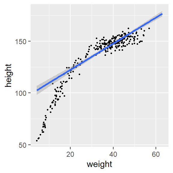

plot(conditional_effects(fit1, "age"),points = TRUE, point_args = list(size = 0.5))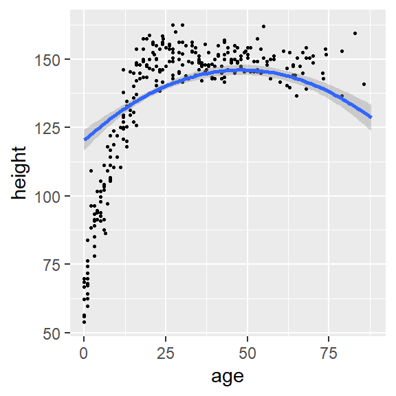

plot(conditional_effects(fit1, "male"))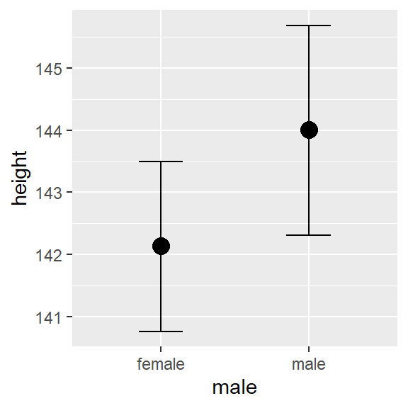

• Coefficient of determination \(R^2\) is the proportion of the variation in the dependent variable that is predictable from the independent variable(s).
  • The estimated \(R^2\) is about 0.9. Really good! About 90% of the variance on height is explained by our model.

bayes_R2(fit1)

##     Estimate   Est.Error      Q2.5     Q97.5
## R2 0.9010756 0.002608764 0.8953755 0.9055377

• predictive intervals
  • predicting height for a female, 33 years of age and weighting 60kg

ind_predic <- posterior_predict(fit1, newdata = data.frame(weight = 60, age = 33, male = "female"))
# mean of the predicted heights
mean(ind_predic)

## [1] 174.3464

# Construct a 95% posterior credible interval
posterior_interval(ind_predic, prob = 0.95)

##          2.5%    97.5%
## [1,] 157.0509 191.5679

# Posterior predictive probability of height > 164
sum(ind_predic>164)/length(ind_predic)

## [1] 0.88075

6.1.3 Model diagnostics

• Geweke index and R-hat (Geweke et al. 1991) to check for MCMC convergence

modelposterior<- as_draws_matrix(fit1)
geweke.diag(modelposterior)

## 
## Fraction in 1st window = 0.1
## Fraction in 2nd window = 0.5 
## 
## b_Intercept    b_weight       b_age    b_IageE2  b_malemale       sigma 
##     1.10099    -0.36665     0.04242    -0.04991    -0.05772    -0.37171 
##        lp__ 
##     1.16552

• Posterior predictive graphic check for model fit
• A “good” Bayesian model produces posterior predicted sets of response values with features similar to the original data.
  • It appears our model can be improved! One suggestion is to fit a non-linear term for weight variable.
  • sometime, people also consider data transformation, e.g., log(height)
  • we can also try using student-t distribution not normal distribution to fit the mean!
  • the observed min and max height is not covered in our posterior predictive samples…

pp_check(fit1, ndraws = 50)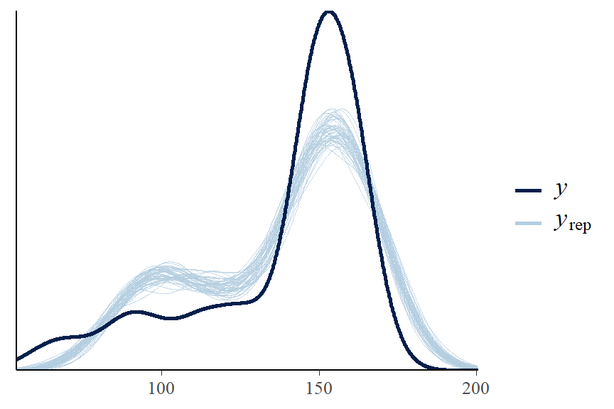

pp_check(fit1, type = "stat_2d", stat = c("max", "min"))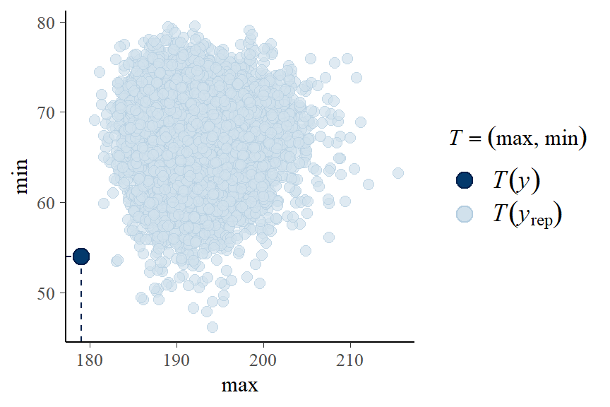

• Residual plot by continuous variables - checking for linearity assumption

res_df <- fit1$data %>% 
  mutate(predict_y = predict(fit1)[ , "Estimate"], 
         std_resid = residuals(fit1, type = "pearson")[ , "Estimate"])
ggplot(res_df, 
       aes(predict_y, std_resid)) + 
  labs(y="Standardized residuals") +
  geom_point(size = 0.8) + stat_smooth(se = FALSE) + theme_bw()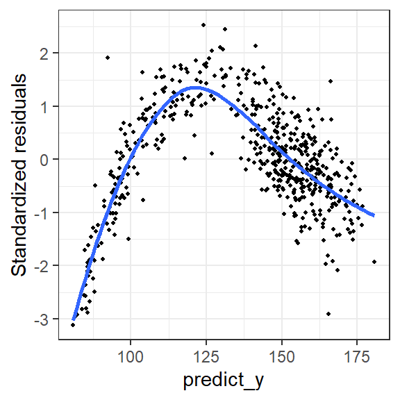

• multicollinearity
  • If some coefficients are particularly strongly correlated, you may need to think about using a stronger prior or combining some predictors.

pairs(fit1, pars = "b", 
      off_diag_args =  # arguments of the scatterplots
        list(size = 0.5,  # point size
             alpha = 0.25))  # transparency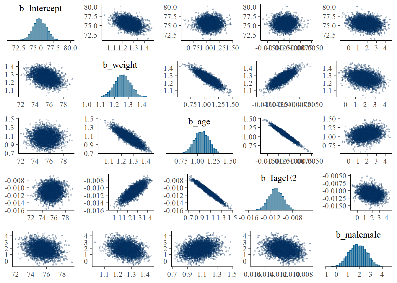

6.1.4 Model comparision

Watanabe-Akaike Information Criteria (WAIC)

• WAIC (Watanabe and Opper 2010) is an alternative approach to DIC in estimating the expected log point-wise predictive density
• The smaller the better!
• WAIC incorporates prior information, and the use of point-wise likelihood makes it more robust when the posterior distributions deviate from normality.
• In general, WAIC is a better estimate of the out-of-sample deviance than AIC and DIC.
• In R under brms package we can use waic() function to obtain WAIC.

Bayesian Leave-one-out cross-validation

• The idea of cross-validation is to split the sample so that it imitates the scenario of estimating the parameters in part of the data and predicting the remaining part.

  • data that are used for estimation is called the training set, and data that are used for prediction is called the validation set.

• Leave-one-out information criteria (LOO-IC) based on posterior predictive distribution

  • means that one uses \(n-1\) observations as the training set and 1 observation as the validation sample, repeat the process \(n\) times so that each time a different observation is being predicted

• LOO-IC requires fitting the model \(n\) times, it is generally very computational intensive

• WAIC can be treated as a fast approximation of LOO-IC, although LOO-IC is more robust and will be a better estimate of out-of-sample deviance

• In R under brms package we can use loo() function to obtain LOO-IC.

Comparing model with \(weight^2\)

• fitting the new model on height, adjusting for age, sex, weight, \(age^2\) and \(weight^2\)
• comparing this model to the regression model adjusted for age, \(age^2\), sex, and weight using WAIC and LOO.

fit2 <- brm(data = dat,
             family = gaussian,
             height ~ weight + I(weight^2) + age + I(age^2) + male, 
             prior = c(prior(normal(0, 100), class = Intercept),
                       prior(normal(0, 10), class = b),
                       prior(gamma(1, 0.01), class = sigma)),
             iter = 20000, 
             warmup = 18000, 
             chains = 4, 
             cores = 4, #instructions on MCMC
             seed = 123, # random number seed to make results reproducible
             silent = 2,
             refresh = 0)
saveRDS(fit2, "data/chp7_height2")

waic1 <- waic(fit1)
waic2 <- waic(fit2)
compare_ic(waic1, waic2) 

loo1 <- loo(fit1)
loo2 <- loo(fit2)
loo_compare(loo1, loo2)

fit2<-readRDS("data/chp7_height2")
pp_check(fit2, ndraws = 50)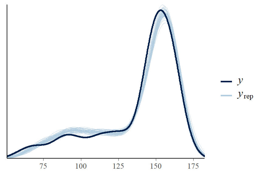

6.2 Hierarchical models

• Often models have more complex structures than the ones described by likelihood and priors and simple relationships between data and parameters

• In these models data and parameters participate in relationships of hierarchical fashion

  • e.g., Correlated and clustering data structures, such as measures within patients, patients within clinics etc.

• Bayesian models deal with hierarchical models in a natural and intuitive way (Bürkner 2017)

• Source of correlation in clustered (or longitudinal) data

  • between-individual heterogeneity on i) mean and ii) velocity (rate of change; slop)
  • Within-individual/cluster homogeneity

Bayesian Hierarchical Models

• Often Bayesian models can we written in the following layers of the hierarchy
  1. Data Layer \(Y \mid \theta\), the likelihood for the observed data \(Y\) given model parameters \(\theta\).
  2. Adaptive/Structural Priors \(\theta \mid \alpha, \beta\), the model for parameter \(\theta\) that defined by the latent data generating process governed by the hyperparameters \(\alpha\) and \(\beta\)
  3. Hyper Priors \(\alpha\) and \(\beta\) as hyper parameters.

Let’s look at a hospital mortality study as an example. This data capture hospital mortality for a specific condition at 20 different hospitals. There is also a variable that describes the average severity of patients at each hospital.

• First let’s examine the data

dat <- read.table("data/HospitalMortality.csv",sep=",", header=T)

dat <- dat %>% 
  mutate(Hospital = factor(Hospital),
         Prop.Dead = round(Deaths/N,3))

dat %>% datatable(
  rownames = FALSE,
  options = list(
    columnDefs = list(list(className = 'dt-center', 
                      targets = 0:4))))

dat %>% select(Severity, Prop.Dead) %>% tbl_summary()

Characteristic	N = 251
Severity	4.10 (3.60, 4.60)
Prop.Dead	0.05 (0.04, 0.08)
1 Median (IQR)

1. First model - considering independent between hospital mortality

• We are modelling \[Deaths_i \sim Bin(p_i, n_i)\], where \(i = 1, \ldots, 25\) and \(p_i\) represent the risk of death for the \(i\) hospital with a beta(1,1) prior on all \(p_i\)s
• This model is saying that there is nothing to link mortality in hospital 1 to mortality in any other hospital
  • We are essentially estimating the risk of mortality for each hospital

fit1 <- brm(data = dat,
            family= binomial,
            Deaths | trials(N) ~ 0 + Hospital,  
            iter = 10000,
            warmup = 8000,
            chains = 4,
            cores = 4, 
            seed = 123, 
            silent = 2,
            refresh = 0)
# saveRDS(fit1, "data/chap7_h_example1")

• Summarizing posterior results

fit1 <- readRDS("data/chap7_h_example1")
#posterior summary of risk (table);
round(exp(fixef(fit1)),3)

##            Estimate Est.Error  Q2.5 Q97.5
## Hospital1     0.022     1.609 0.008 0.051
## Hospital2     0.071     2.257 0.012 0.283
## Hospital3     0.041     1.337 0.022 0.070
## Hospital4     0.024     1.881 0.006 0.066
## Hospital5     0.010     3.566 0.000 0.064
## Hospital6     0.042     1.494 0.018 0.086
## Hospital7     0.018     3.728 0.001 0.124
## Hospital8     0.047     1.913 0.011 0.143
## Hospital9     0.041     1.728 0.012 0.105
## Hospital10    0.035     1.350 0.019 0.061
## Hospital11    0.051     1.389 0.026 0.093
## Hospital12    0.133     1.472 0.058 0.270
## Hospital13    0.109     1.238 0.071 0.164
## Hospital14    0.081     1.249 0.051 0.122
## Hospital15    0.045     1.500 0.019 0.093
## Hospital16    0.329     1.279 0.200 0.527
## Hospital17    0.301     1.159 0.224 0.398
## Hospital18    0.034     1.629 0.012 0.079
## Hospital19    0.066     1.430 0.031 0.125
## Hospital20    0.082     1.317 0.046 0.136
## Hospital21    0.064     1.415 0.031 0.122
## Hospital22    0.085     1.289 0.050 0.137
## Hospital23    0.035     1.493 0.015 0.070
## Hospital24    0.017     1.920 0.004 0.051
## Hospital25    0.044     1.420 0.021 0.083

#posterior summary of risk (visual);
mcmc_intervals(fit1, transformations = "plogis")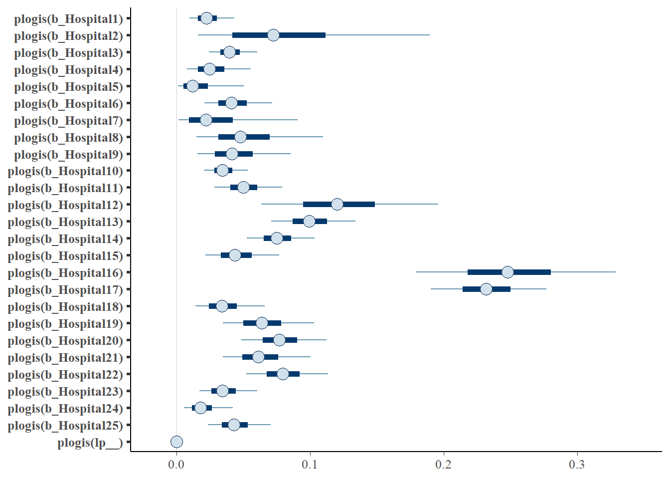

2. Second model - shared parameters on hospital mortality (complete pooling)

• Suppose that these were 25 hospitals in the same city

  • Similar practices, populations, shared staff in some cases

• How can we treat them as one big hospital with exactly the same mortality?

  • Easy - specify in the model that they share the same probability \(p\)

• Parameterizing using odds

  • Odds are the basis for logistic regression, where we model log(odds)
  • \(0 \leq p \leq 1 \Rightarrow - \infty \leq \log(Odds) \leq \infty\)
  • Suggests an normal uninformative prior on log odds with a sufficient variance (ie sd = 10)

  \[ \log(Odds) \sim N(0,\sigma^2)\]

• Assume a common odds between all 25 hospitals, we run a pooled model such that \[Deaths_i \sim Bin(p, n_i)\]. This is a complete pooling model.

• We are essentially modelling the average population risk of mortality pooling information from all 25 hospitals.

fit1.p <- brm(data = dat,
            family= binomial,
            Deaths | trials(N) ~ 1,  
            iter = 10000,
            warmup = 8000,
            chains = 4,
            cores = 4, 
            seed = 123, 
            silent = 2,
            refresh = 0)
# saveRDS(fit1.p, "data/chap7_h_example1p")

• Summarizing posterior results

##           Estimate Est.Error  Q2.5 Q97.5
## Intercept    0.074     1.063 0.066 0.083

• Drawbacks of a complete pooling approach

There are two main drawbacks to taking a complete pooling approach to analyze group structured data:

• in case of clustered and correlated data, we violate the assumption of independence
• misleading conclusions about the relationship between and across subjects

3. third model - shared parameters on hospital mortality (partial pooling)

• Suppose that these were 25 hospitals in the same city

  • Similar (but not same) practices and patient populations; partly shared staff

• How can we treat them as similar

  • with a common underlying true mortality
  • with random variation from hospital to hospital in the true mortality!

• Need to introduce two parameters representing

  • Common mortality (mean log odds)
  • Hospital-to-hospital variation (sd of log odds)

• This introduces an hierarchical structure in the model!

• Specifically, we have

  1. Data Layer \(y_i \mid p_i \sim P(y_i \mid p_i)\)
  2. Adaptive/Structural Priors \(logit(p_i) \mid \theta, \sigma^2 \sim P(logit(p_i) \mid \theta, \sigma^2)\)
  3. Hyper Priors \(\theta \sim P(\theta)\) and \(\sigma^2 ~ P(\sigma^2)\) as hyper parameters.

• A Bayesian random intercept model!

fit1.ri <- brm(data = dat,
            family= binomial,
            Deaths | trials(N) ~ 1 + (1|Hospital),  
            iter = 10000,
            warmup = 8000,
            chains = 4,
            cores = 4, 
            seed = 123, 
            silent = 2,
            refresh = 0)
# saveRDS(fit1.ri, "data/chap7_h_example1ri")

• Summarizing posterior results on risk and between-hospital standard deviation of the intercept

fit1.ri <- readRDS("data/chap7_h_example1ri")
summary(fit1.ri)

##  Family: binomial 
##   Links: mu = logit 
## Formula: Deaths | trials(N) ~ 1 + (1 | Hospital) 
##    Data: dat (Number of observations: 25) 
##   Draws: 4 chains, each with iter = 10000; warmup = 8000; thin = 1;
##          total post-warmup draws = 8000
## 
## Group-Level Effects: 
## ~Hospital (Number of levels: 25) 
##               Estimate Est.Error l-95% CI u-95% CI Rhat Bulk_ESS Tail_ESS
## sd(Intercept)     0.71      0.13     0.49     1.01 1.00     3005     4847
## 
## Population-Level Effects: 
##           Estimate Est.Error l-95% CI u-95% CI Rhat Bulk_ESS Tail_ESS
## Intercept    -2.82      0.17    -3.15    -2.50 1.00     2301     3937
## 
## Draws were sampled using sampling(NUTS). For each parameter, Bulk_ESS
## and Tail_ESS are effective sample size measures, and Rhat is the potential
## scale reduction factor on split chains (at convergence, Rhat = 1).

#posterior summary of risk overall (table);
round(exp(fixef(fit1.ri)),3)

##           Estimate Est.Error  Q2.5 Q97.5
## Intercept     0.06      1.18 0.043 0.082

s1 <- posterior_samples(fit1.ri)
sigma <- s1[,"sd_Hospital__Intercept"]
qs <- quantile(sigma,c(0.025, 0.975))

temp <- density(sigma,n = 1024)
dp1 <- data.frame(sigma=temp$x, density=temp$y, area=cut(temp$x, c(0,qs,10), include.lowest = T))

ggplot(dp1, aes(x=sigma, y=density))+geom_area(aes(fill=area), show.legend=FALSE)+
    theme_bw()+
    geom_line(color="orange")+
    ggtitle(paste0("Mean sigma= ", round(mean(sigma),2),"; 95% CrI: ", round(qs[1],1),
                   " to ",round(qs[2],2)))+
    scale_fill_manual(values=c("orange","white","orange"))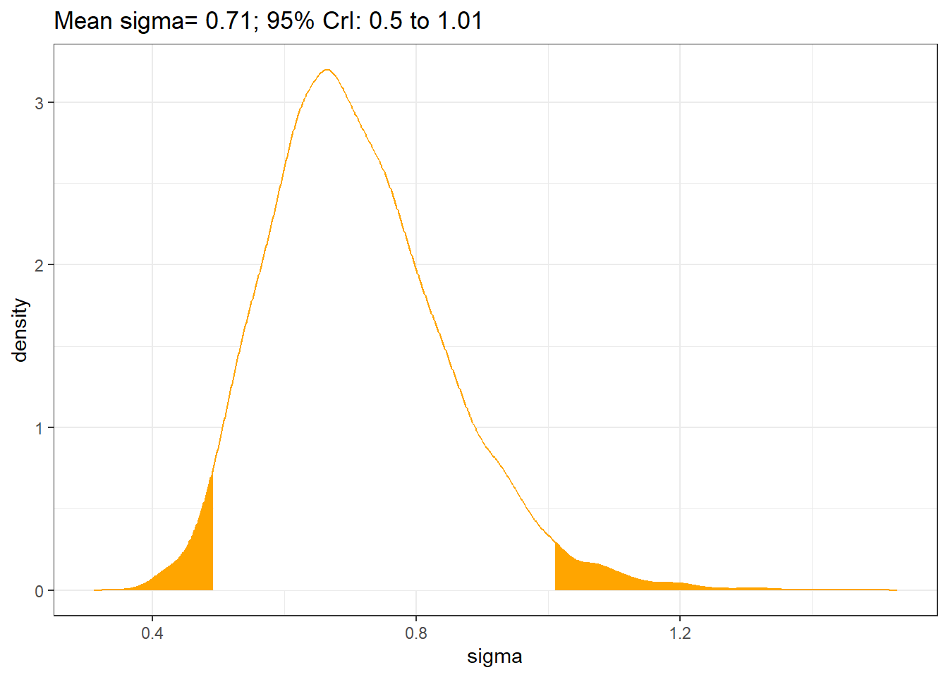

• Hospitals, ranked best to worst by posterior odds of mortality (median ranking on mortality, along with a 95% CrI)

h <- s1[,grep(",Intercept",names(s1))]
r <- apply(h,1,rank)
rankings <- t(apply(r,1,quantile, c(0.5, c(0.025, 0.975))))
row.names(rankings) <- paste("Hospital",1:25)
colnames(rankings)[1] <- "Median"
rankings <- data.frame(rankings, ObservedProportion=round(dat$Deaths/dat$N,3), n=dat$N)
rankings <- rankings[order(rankings[,1]),]
knitr::kable(rankings, caption="Hospitals, ranked best to worst by posterior odds of mortality")

Table 6.1: Hospitals, ranked best to worst by posterior odds of mortality

	Median	X2.5.	X97.5.	ObservedProportion	n
Hospital 1	4	1	14	0.024	209
Hospital 24	4	1	15	0.020	149
Hospital 5	5	1	20	0.017	60
Hospital 4	6	1	18	0.028	109
Hospital 10	7	1	15	0.035	340
Hospital 23	7	1	18	0.036	196
Hospital 18	8	1	19	0.036	140
Hospital 3	9	2	17	0.041	319
Hospital 6	10	2	20	0.043	164
Hospital 7	10	1	22	0.031	32
Hospital 9	11	1	21	0.045	89
Hospital 15	11	2	20	0.046	153
Hospital 25	11	2	19	0.044	203
Hospital 8	13	2	23	0.053	57
Hospital 11	13	3	21	0.051	196
Hospital 19	16	5	22	0.065	138
Hospital 21	16	5	22	0.063	142
Hospital 2	17	2	23	0.083	24
Hospital 14	18	11	23	0.076	290
Hospital 20	19	10	23	0.078	192
Hospital 22	19	11	23	0.081	211
Hospital 12	22	12	23	0.123	65
Hospital 13	22	16	23	0.100	250
Hospital 16	24	24	25	0.250	92
Hospital 17	25	24	25	0.232	267

6.2.1 Clustered data (Multi-level)

• Example: Developmental toxicity study of ethylene glycol (EG) (Price et al. 1985)

• The data are from a development toxicity study of ethylene glycol (EG).

• Ethylene glycol is a high-volume industrial chemical used in many applications.

• In a study of laboratory mice conducted through the National Toxicology Program (NTP), EG was administered at doses of 0, 750, 1500, or 3000 mg/kg/day to 94 pregnant mice (dams) over the period of major organogenesis, beginning just after implantation.

• Following sacrifice, fetal weight and evidence of malformations were recorded

• Let’s first read in the data

  • This data set is in a long format
  • we can see each row represents a mouse.
  • Mice are nested within the litter. We have a two-level data!

ntp <- read.table("data/ntp-data.txt", header = TRUE)
colnames(ntp) <- c("Litter", "Dose", "Weight", "Malformation")
ntp <- ntp %>%
  group_by(Litter) %>%
  mutate(Litid = row_number()) %>% # seq id for each litter
  mutate(FetalID = paste0(Litter, ".", Litid)) %>% # FetalID = LitID.tempid
  select(-Litid) # remove tempid from toxic2
knitr::kable(head(ntp), row.names = F)

Litter	Dose	Weight	Malformation	FetalID
60	0	0.828	0	60.1
60	0	0.953	0	60.2
60	0	0.954	0	60.3
60	0	1.070	0	60.4
60	0	1.065	0	60.5
60	0	0.959	0	60.6

• Number of doses in each group and number of fetuses in each litter

cluster <- ntp %>% group_by(Dose) %>%
  summarize(nlitter = n_distinct(Litter), nfetal = n_distinct(FetalID))
cluster %>% datatable(
  rownames = FALSE,
  options = list(
    columnDefs = list(list(className = 'dt-center', 
                      targets = 0:2))))

clustersize <- ntp %>% group_by(Litter) %>% summarise(csize = n_distinct(FetalID))
# clustersize %>% datatable(
#   rownames = FALSE,
#   options = list(
#     columnDefs = list(list(className = 'dt-center', 
#                       targets = 0:1))))

clustersize %>%
ggplot(aes(x = Litter, y = csize)) +
geom_bar(stat = "identity", fill = "black", color = "snow1")+
  theme_bw()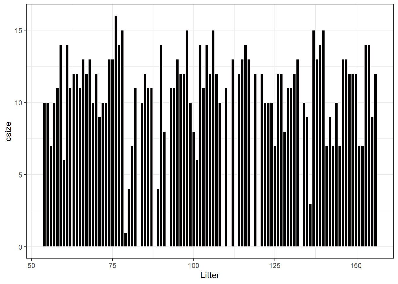

• Visualize relationship between fetal malformation and dose

ntp %>%
  group_by(Dose, Litter) %>%
  summarise(fmalprop = mean(Malformation)) %>%
  ggplot(aes(x = Litter, y = fmalprop)) +
  geom_bar(stat = "identity", fill = "steelblue") +
  ylab("Proportion of Malformation")+
  facet_wrap(~Dose)+
  theme_bw()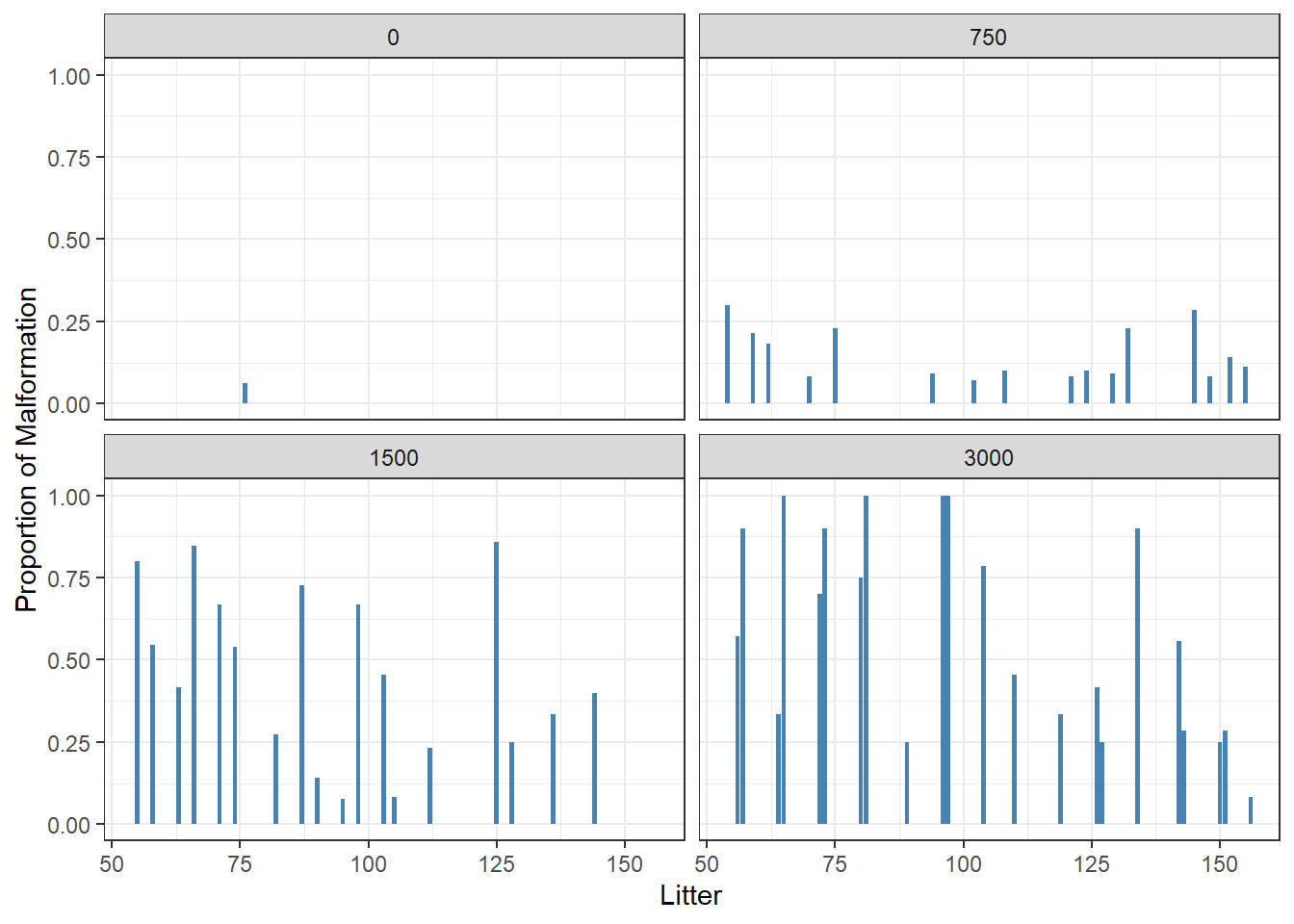

• Visualize relationship between fetal weight and dose

ntp %>%
  ggplot(aes(x = Litter, y = Weight)) +
  geom_boxplot(aes(group = Litter), color = "steelblue") +
  facet_wrap(~Dose)+
  theme_bw()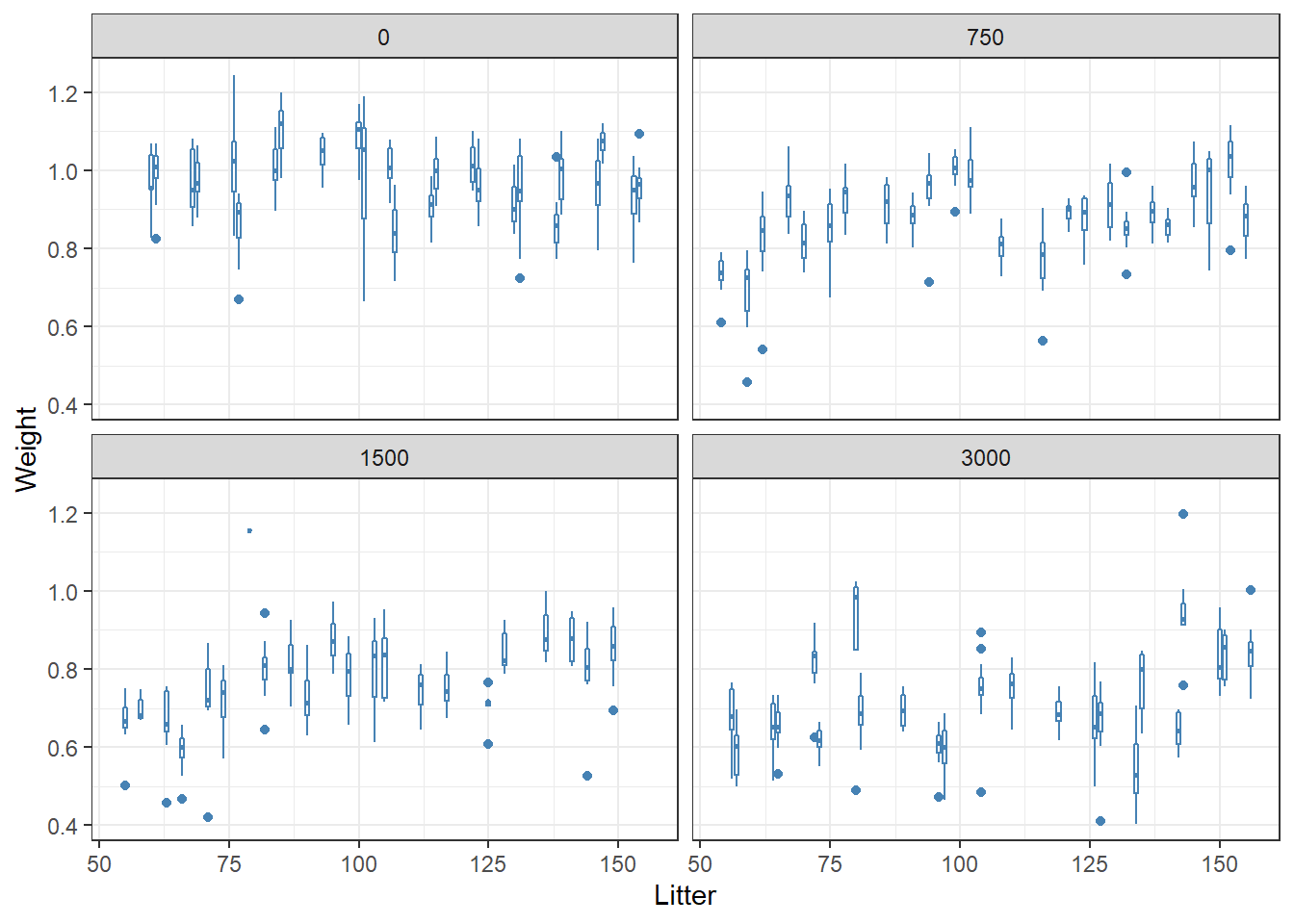

ntp <- ntp %>% 
  mutate(Dose = factor(Dose, levels = c("0","750","1500","3000")))

• Suppose we are interested to assess the effect of dose on fetal weight.

• The data on fetal weight from this experiment are clustered, with observations on the fetuses nested within litters.

• First model - Normal hierarchical model with random intercept

• data structure: model of fetal weight within each litter (index by j) \[ Y_{ij} \mid \mu_j, \sigma_y \sim N(\mu_j, \sigma_y^2)\]

• adaptive priors on litter-level mean

\[\mu_j \mid \mu, \sigma_\mu \sim N(\mu, \sigma_u^2)\]

• hyperparameter priors on \(\mu\), \(\sigma_u\) as well as global prior for \(\sigma_y\)

• Variability within litter by dose

  • in this model, only \(\beta_{0j}\) depends on litter
  • \(\beta_{1}\) is shared across all litter \(j\), the expected change in fetal weight comparing between various dosage to reference level (dose = 0)
  • \(\sigma_y\) measures Within-group variability around the mean regression model \(\beta_{0j} + \beta_{1} \ dose_{ij}\)

\[\mu_{ij} = \beta_{0j} + \beta_{1} \ dose_{ij}\]

• specifying our hierarchical random intercepts model (update with \(\beta\)):

\[ Y_{ij} \mid \beta_{0j}, \beta_{1}, \sigma_y \sim N(\beta_{0j} + \beta_{1} \ dose_{ij}, \sigma_y^2) \]

\[\beta_{0j} \mid \beta_{0}, \sigma_0^2\]

\[\beta_{0} \sim N(0,10)\] \[\beta_{1} \sim N(0,10)\] \[\sigma_y \sim HalfCauchy(10)\] \[\sigma_0 \sim HalfCauchy(10)\]

fit2 <- brm(data = ntp,
            family= gaussian(),
            Weight ~ Dose + (1|Litter),  
            prior = c(prior(normal(0, 10), class = Intercept),
                      prior(normal(0, 10), class = b),
                      prior(cauchy(0, 10), class = sd),
                      prior(cauchy(0, 10), class = sigma)),
            iter = 10000,
            warmup = 8000,
            chains = 4,
            cores = 4, 
            seed = 123, 
            silent = 2,
            refresh = 0)
# saveRDS(fit2, "data/chap7_h_example2")

fit2 <- readRDS("data/chap7_h_example2")
summary(fit2)

##  Family: gaussian 
##   Links: mu = identity; sigma = identity 
## Formula: Weight ~ Dose + (1 | Litter) 
##    Data: ntp (Number of observations: 1027) 
##   Draws: 4 chains, each with iter = 10000; warmup = 8000; thin = 1;
##          total post-warmup draws = 8000
## 
## Group-Level Effects: 
## ~Litter (Number of levels: 94) 
##               Estimate Est.Error l-95% CI u-95% CI Rhat Bulk_ESS Tail_ESS
## sd(Intercept)     0.09      0.01     0.07     0.10 1.00      991     1619
## 
## Population-Level Effects: 
##           Estimate Est.Error l-95% CI u-95% CI Rhat Bulk_ESS Tail_ESS
## Intercept     0.97      0.02     0.94     1.01 1.01      692     1418
## Dose750      -0.09      0.03    -0.14    -0.04 1.00      808     1647
## Dose1500     -0.19      0.03    -0.24    -0.14 1.00      974     2217
## Dose3000     -0.26      0.03    -0.31    -0.21 1.00      794     1737
## 
## Family Specific Parameters: 
##       Estimate Est.Error l-95% CI u-95% CI Rhat Bulk_ESS Tail_ESS
## sigma     0.07      0.00     0.07     0.08 1.00     6968     5538
## 
## Draws were sampled using sampling(NUTS). For each parameter, Bulk_ESS
## and Tail_ESS are effective sample size measures, and Rhat is the potential
## scale reduction factor on split chains (at convergence, Rhat = 1).

# checking traceplot
# fit2 %>% plot( combo = c("hist", "trace"), widths = c(1, 1.5),
#       theme = theme_bw(base_size = 10))
conditional_effects(fit2)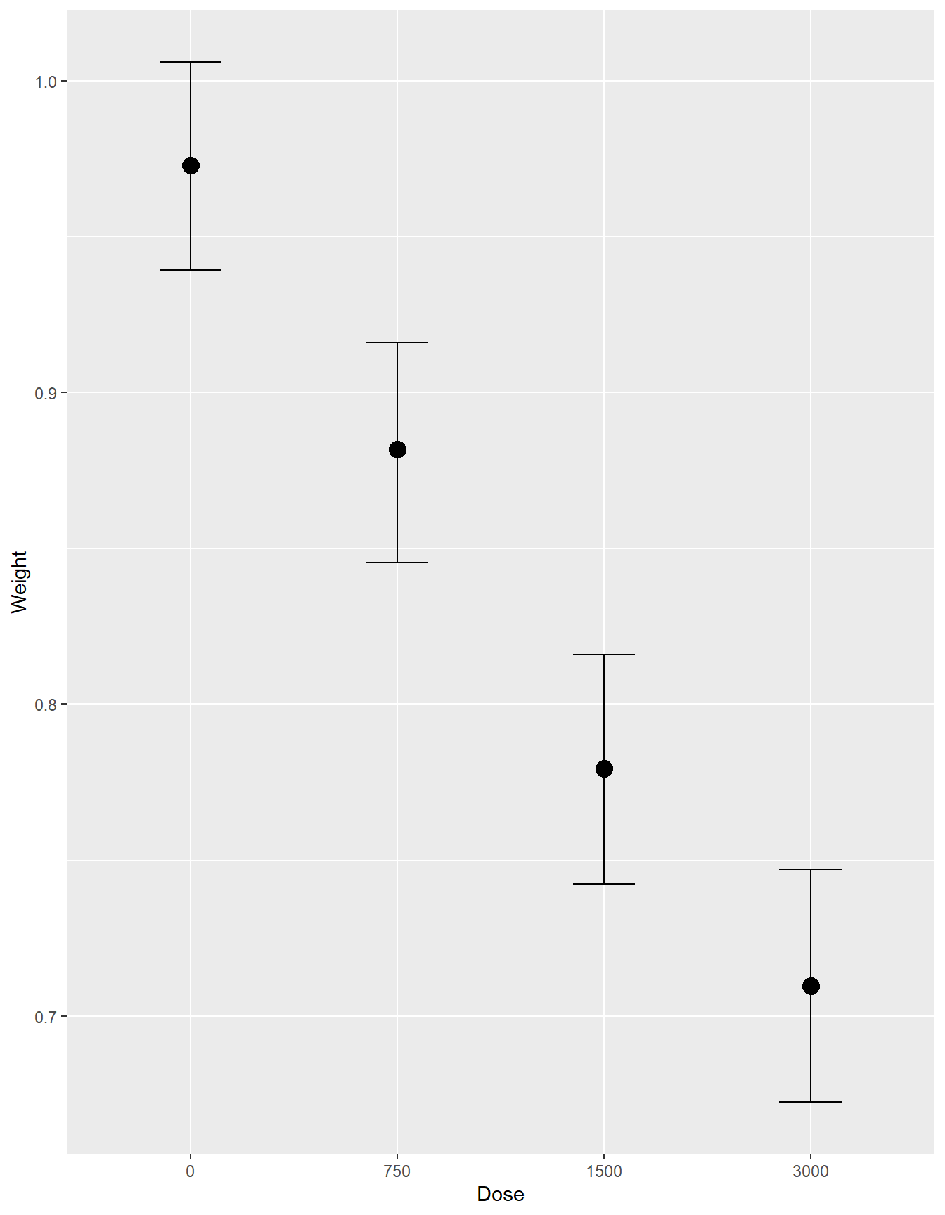

• The adjusted ICC represents the proportion of variance of the outcome that are due to between-level (e.g., between-group, between-person) differences
  • Does not consider fixed effect! In this case, adjusted ICC does not feature variation caused by dose.

\[\rho_{adj} = \frac{\sigma_0^2}{\sigma_0^2 + \sigma^2}\]

• where \(\sigma_0^2\) is the between-level SD, which is the SD of cluster means (i.e., variability between litters) and \(\sigma\) is the observation-specific SD (i.e., variability within a litter)

• The conditional ICC considers variation with fixed effect, in this case dose.

\[\rho_{c} = \frac{\sigma_0^2}{\sigma_0^2 + \sigma^2 + \sigma_f^2}\]

\[\sigma_f^2 = var(\sum_{m=1}^p \beta_m x_{mij}), p \text{ # of coefficients exclude } \beta_0\]

• reference: (Nakagawa, Johnson, and Schielzeth 2017) doi: 10.1098/rsif.2017.0213

• We can use the posterior draws of the two SD to compute the posterior for the adjusted ICC:

# Computing ICC
# 1. Obtain posterior draws of tau and sigma
sd_m2 <- VarCorr(fit2, summary = FALSE)
draws_tau <- sd_m2$Litter$sd[ , "Intercept"]  # tau
draws_sigma <- sd_m2$residual__$sd[ , 1]  #sigma
# 2. Compute draws for adjusted ICC
draws_icc <- draws_tau^2 / (draws_tau^2 + draws_sigma^2)
# quantile of posterior adjusted ICC
quantile(draws_icc, p=c(0.5, 0.025,0.975))   

##       50%      2.5%     97.5% 
## 0.5623851 0.4789231 0.6524716

# Plot the adjusted ICC
qplot(draws_icc, geom = "density", xlab = "ICC adjust", bw = "SJ")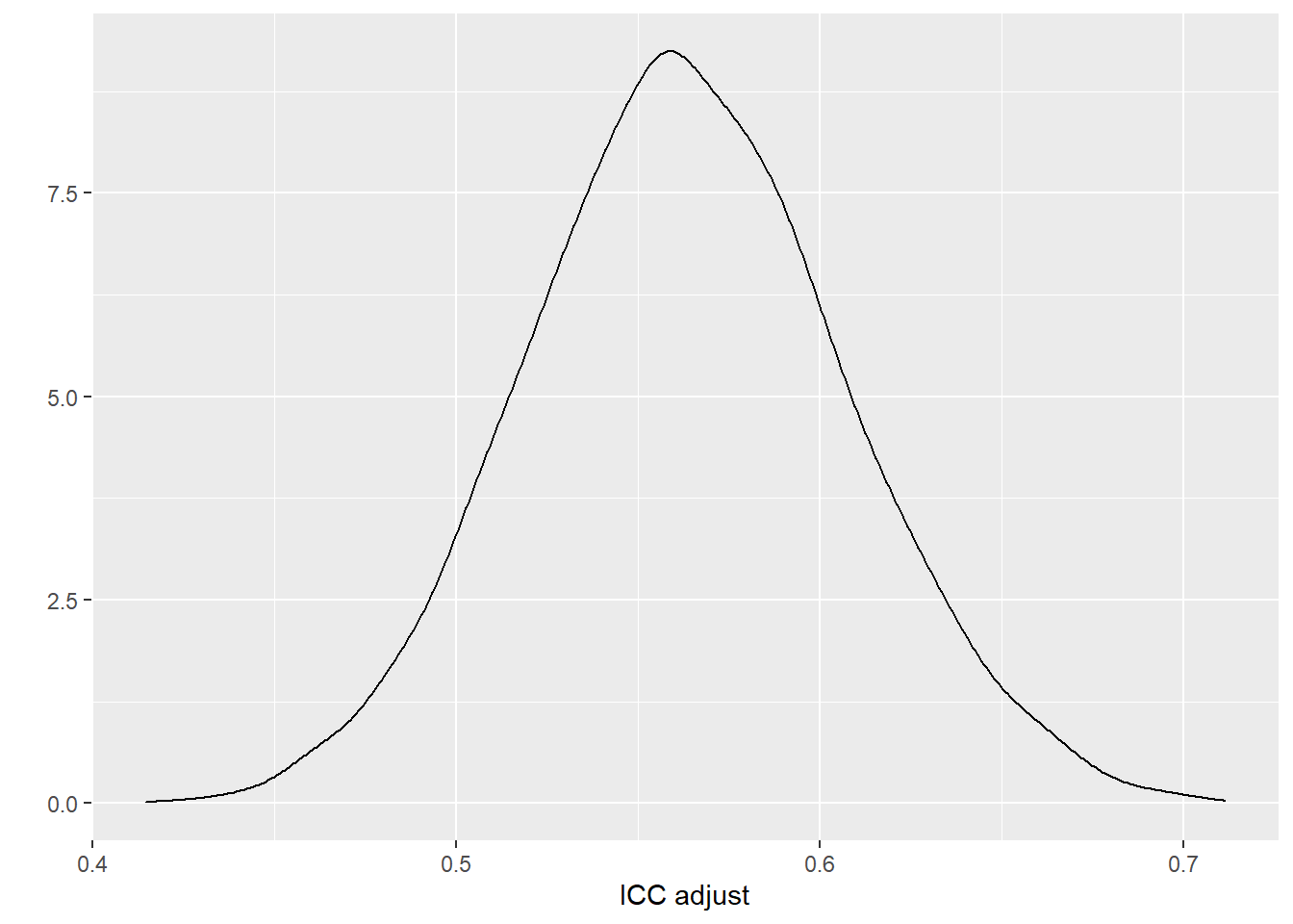

• It was estimated that 56%, 95% CI [48%, 65%] of the variations in fetal weight was attributed to between-litter differences.

• We can use the posterior draws of b_Dose750, b_Dose1500, and b_Dose3000 (fix effects) to compute the posterior for the conditional ICC:

# sjstats::icc(fit2) point estimate of adjusted and conditional ICC;
# Intraclass Correlation Coefficient
# 
#      Adjusted ICC: 0.565
#   Conditional ICC: 0.317

# calculating conditional ICC
post_par <- colMeans(posterior_samples(fit2, pars = c("b_Dose750","b_Dose1500","b_Dose3000")))
dummy <- with(ntp, outer(Dose, levels(Dose), `==`)*1)[,-1] #dummy matrix removing dose0 level;
sigma_f2 <- var(dummy%*%post_par)
draws_icc_conditional <- (draws_tau^2) / (draws_tau^2 + sigma_f2+ draws_sigma^2)
# quantile of posterior conditional ICC
quantile(draws_icc_conditional, p=c(0.5, 0.025,0.975)) 

##       50%      2.5%     97.5% 
## 0.3142783 0.2486054 0.3974582

# Plot the adjusted ICC
qplot(draws_icc_conditional, geom = "density", xlab = "ICC conditional", bw = "SJ")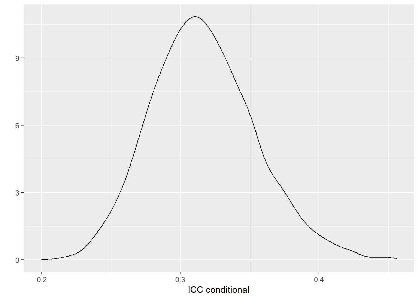

• It was estimated that 31%, 95% CI [25%, 40%] of the variations in fetal weight was attributed to between-litter differences given fix effects.

• Second model - Normal hierarchical model with varying intercept and slope

• Variability in “velocity” between individual, dose the effect of dose on weight also vary by litter?

• We want to build a model which recognizes that in the relationship between feta weight and dose,

  • where the intercept (i.e., baseline weight)
  • and slope (i.e., rate at which weight changes with dose) might vary from mouse to mouse.

• A random intercept and slope model!

• Variability within litter by dose

  • in this model, \(\beta_{0j}\) and \(\beta_{1j}\) depend on litter

• specifying our hierarchical random intercept and slope model :

\[ Y_{ij} \mid \beta_{0j}, \beta_{1j}, \sigma_y \sim N(\beta_{0j} + \beta_{1j} \ dose_{ij}, \sigma_y^2) \]

\[\beta_{0j} \mid \beta_{0}, \sigma_0^2\] \[\beta_{1j} \mid \beta_{1}, \sigma_1^2\]

• In this model \(\beta_{0j}\) and \(\beta_{1j}\) working together to describe the model for litter \(j\), and thus are correlated!

• Let \(\rho \in [-1,1]\) represents the correlation between \(\beta_{0j}\) and \(\beta_{1j}\). We can assign a joint Normal model of \(\beta_{0j}\) and \(\beta_{1j}\) where

\[ \begin{pmatrix} \beta_{0j}\\ \beta_{1j} \end{pmatrix} \mid \beta_{0}, \beta_{1}, \sigma_0, \sigma_1 \sim N(\begin{pmatrix} \beta_{0}\\ \beta_{1} \end{pmatrix}, \begin{pmatrix} \sigma_0^2 & \rho \sigma_0\sigma_1 \\ \rho \sigma_0\sigma_1 & \sigma_1^2 \end{pmatrix}). \]

\[\beta_{0} \sim N(0,10)\] \[\beta_{1} \sim N(0,10)\] \[\sigma_y \sim HalfCauchy(10)\] \[\sigma_0 \sim HalfCauchy(10)\] \[\sigma_1 \sim HalfCauchy(10)\] \[\mathbf{R} \sim LKJcorr(2)\]

• where \(\mathbf{R}\) is the correlation matrix \[\begin{pmatrix} 1 & \rho \\ \rho & 1 \end{pmatrix}\]

• LKJ-correlation prior (Lewandowski, Kurowicka, and Joe 2009) with one parameter (\(\zeta\)) that controls the strength of the correlation.

dlkjcorr2 <- function(rho, eta = 1, log = FALSE) {
  # Function to compute the LKJ density given a correlation
  out <- (eta - 1) * log(1 - rho^2) - 
    1 / 2 * log(pi) - lgamma(eta) + lgamma(eta + 1 / 2)
  if (!log) out <- exp(out)
  out
}
ggplot(tibble(rho = c(-1, 1)), aes(x = rho)) + 
  stat_function(fun = dlkjcorr2, args = list(eta = 0.1), 
                aes(col = "0.1"), n = 501) + 
  stat_function(fun = dlkjcorr2, args = list(eta = 0.5), 
                aes(col = "0.5"), n = 501) + 
  stat_function(fun = dlkjcorr2, args = list(eta = 1), 
                aes(col = "1"), n = 501) + 
  stat_function(fun = dlkjcorr2, args = list(eta = 2), 
                aes(col = "2"), n = 501) + 
  stat_function(fun = dlkjcorr2, args = list(eta = 10), 
                aes(col = "10"), n = 501) + 
  stat_function(fun = dlkjcorr2, args = list(eta = 100), 
                aes(col = "100"), n = 501) + 
  labs(col = expression(eta), x = expression(rho), y = "Density")+
  theme_bw()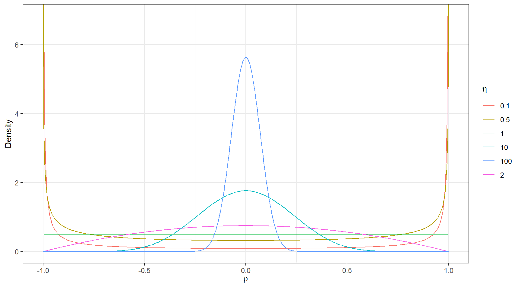

Figure 6.3: LKJ prior for different values of the shape paramete

fit3 <- brm(data = ntp,
            family= gaussian(),
            Weight ~ Dose + (Dose|Litter),  
            prior = c(prior(normal(0, 10), class = Intercept),
                      prior(normal(0, 10), class = b),
                      prior(cauchy(0, 10), class = sd),
                      prior(cauchy(0, 10), class = sigma),
                      prior(lkj(2), class = cor)),
            iter = 11000,
            warmup = 10000,
            chains = 3,
            cores = 4, 
            control = list(adapt_delta = .9), 
            seed = 123, 
            silent = 2,
            refresh = 0)
# saveRDS(fit3, "data/chap7_h_example3")

• Posterior summary

fit3 <- readRDS("data/chap7_h_example3")
summary(fit3)

##  Family: gaussian 
##   Links: mu = identity; sigma = identity 
## Formula: Weight ~ Dose + (Dose | Litter) 
##    Data: ntp (Number of observations: 1027) 
##   Draws: 3 chains, each with iter = 11000; warmup = 10000; thin = 1;
##          total post-warmup draws = 3000
## 
## Group-Level Effects: 
## ~Litter (Number of levels: 94) 
##                         Estimate Est.Error l-95% CI u-95% CI Rhat Bulk_ESS
## sd(Intercept)               0.07      0.01     0.05     0.09 1.01      636
## sd(Dose750)                 0.05      0.03     0.00     0.12 1.00      231
## sd(Dose1500)                0.07      0.04     0.01     0.15 1.00      404
## sd(Dose3000)                0.08      0.04     0.01     0.15 1.01      412
## cor(Intercept,Dose750)     -0.07      0.35    -0.69     0.64 1.00      564
## cor(Intercept,Dose1500)    -0.03      0.36    -0.71     0.66 1.00      647
## cor(Dose750,Dose1500)      -0.01      0.37    -0.69     0.68 1.01     1110
## cor(Intercept,Dose3000)     0.01      0.36    -0.66     0.68 1.01      560
## cor(Dose750,Dose3000)      -0.00      0.37    -0.68     0.70 1.00     1224
## cor(Dose1500,Dose3000)      0.00      0.38    -0.70     0.70 1.00      831
##                         Tail_ESS
## sd(Intercept)               1333
## sd(Dose750)                  708
## sd(Dose1500)                 830
## sd(Dose3000)                 759
## cor(Intercept,Dose750)       790
## cor(Intercept,Dose1500)      653
## cor(Dose750,Dose1500)       1778
## cor(Intercept,Dose3000)      749
## cor(Dose750,Dose3000)       1876
## cor(Dose1500,Dose3000)      1553
## 
## Population-Level Effects: 
##           Estimate Est.Error l-95% CI u-95% CI Rhat Bulk_ESS Tail_ESS
## Intercept     0.98      0.01     0.95     1.00 1.00      855     1252
## Dose750      -0.09      0.02    -0.14    -0.05 1.00     1280     1737
## Dose1500     -0.20      0.03    -0.25    -0.14 1.00     1536     1698
## Dose3000     -0.26      0.03    -0.32    -0.21 1.00     1581     1979
## 
## Family Specific Parameters: 
##       Estimate Est.Error l-95% CI u-95% CI Rhat Bulk_ESS Tail_ESS
## sigma     0.07      0.00     0.07     0.08 1.00     4723     2301
## 
## Draws were sampled using sampling(NUTS). For each parameter, Bulk_ESS
## and Tail_ESS are effective sample size measures, and Rhat is the potential
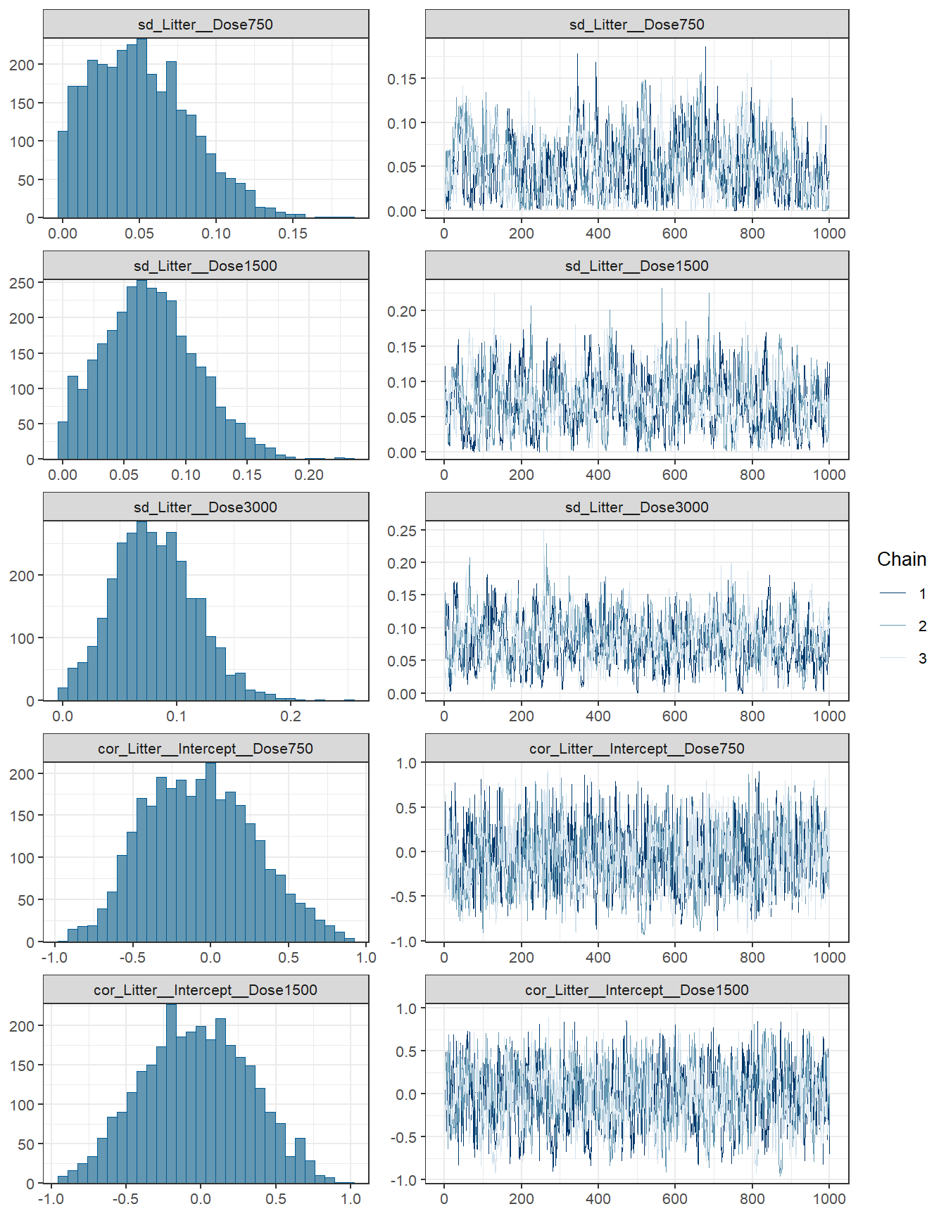
## scale reduction factor on split chains (at convergence, Rhat = 1).

fit3 %>% plot( combo = c("hist", "trace"), widths = c(1, 1.5),
      theme = theme_bw(base_size = 10))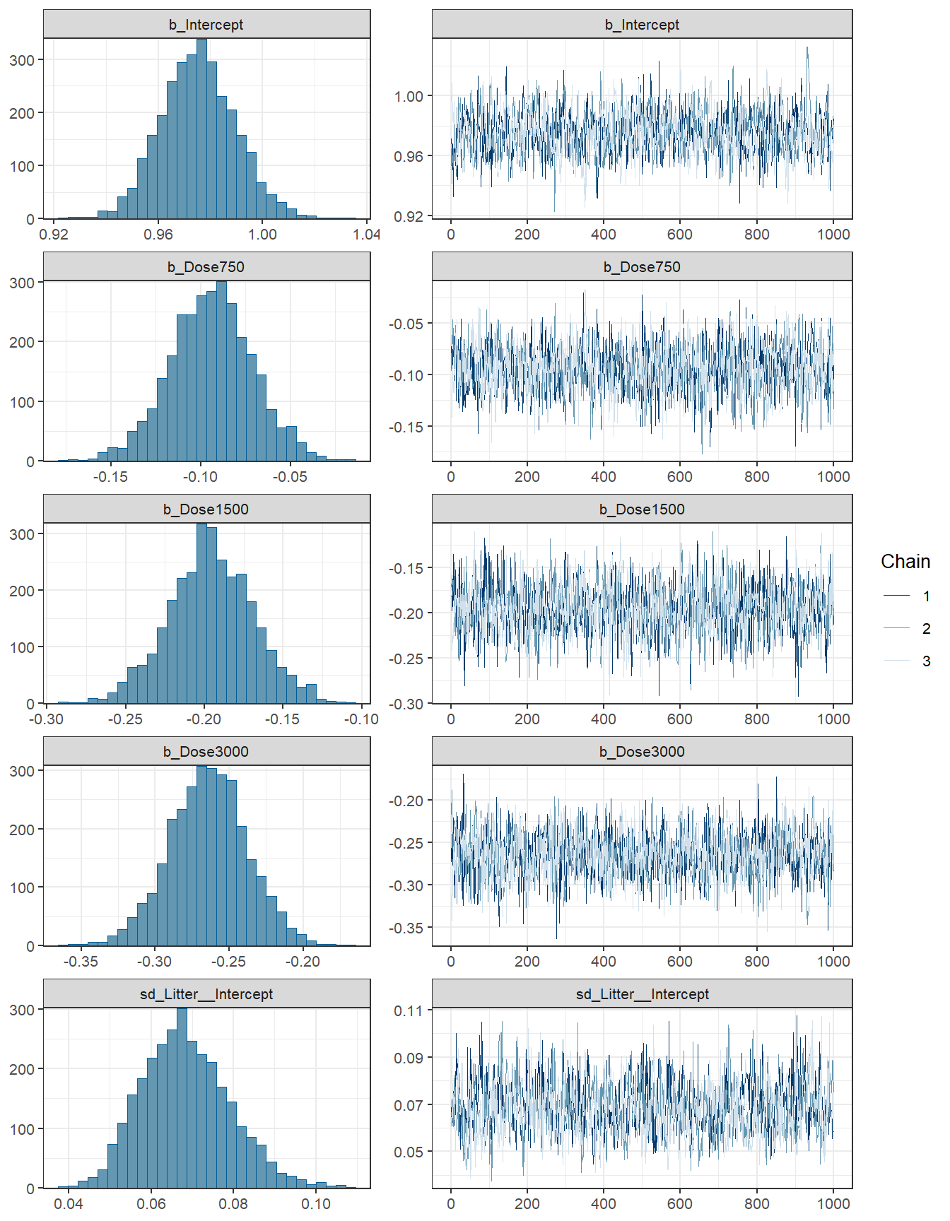

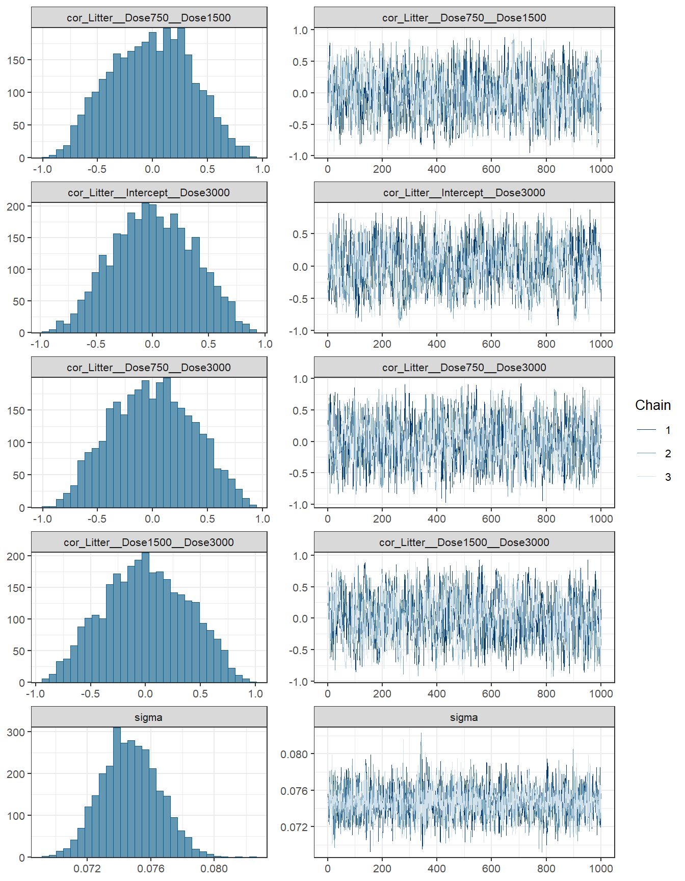
conditional_effects(fit3)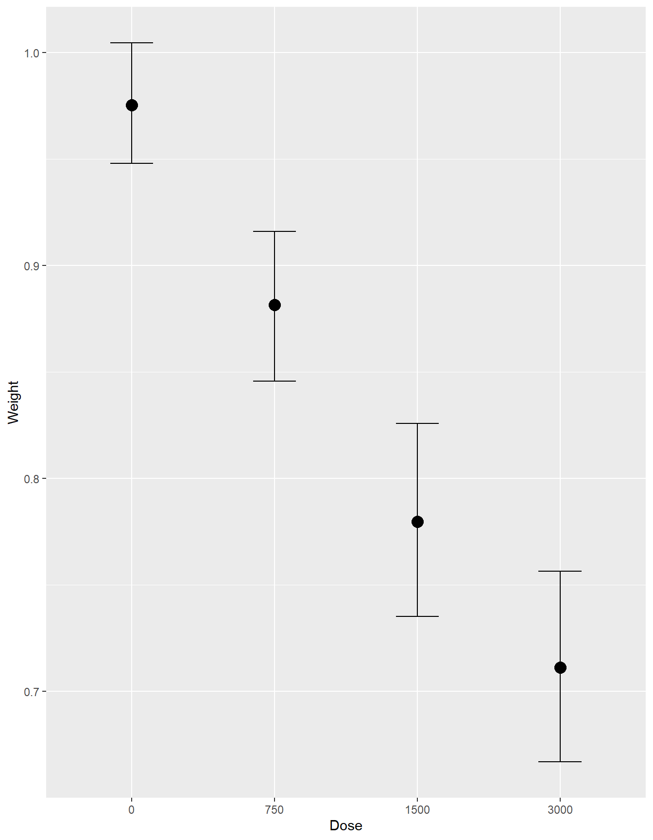

• Interpretations

round(VarCorr(fit3)$Litter$sd, 3)

##           Estimate Est.Error  Q2.5 Q97.5
## Intercept    0.068     0.011 0.050 0.091
## Dose750      0.051     0.032 0.002 0.120
## Dose1500     0.071     0.038 0.006 0.150
## Dose3000     0.080     0.036 0.013 0.155

• Comparing between the two models (both models are really similar)

loo(fit2, fit3)

## Output of model 'fit2':
## 
## Computed from 8000 by 1027 log-likelihood matrix
## 
##          Estimate   SE
## elpd_loo   1153.9 33.6
## p_loo        95.8  8.5
## looic     -2307.9 67.2
## ------
## Monte Carlo SE of elpd_loo is NA.
## 
## Pareto k diagnostic values:
##                          Count Pct.    Min. n_eff
## (-Inf, 0.5]   (good)     1021  99.4%   908       
##  (0.5, 0.7]   (ok)          4   0.4%   183       
##    (0.7, 1]   (bad)         2   0.2%   16        
##    (1, Inf)   (very bad)    0   0.0%   <NA>      
## See help('pareto-k-diagnostic') for details.
## 
## Output of model 'fit3':
## 
## Computed from 3000 by 1027 log-likelihood matrix
## 
##          Estimate   SE
## elpd_loo   1154.2 33.7
## p_loo        96.5  9.0
## looic     -2308.5 67.5
## ------
## Monte Carlo SE of elpd_loo is NA.
## 
## Pareto k diagnostic values:
##                          Count Pct.    Min. n_eff
## (-Inf, 0.5]   (good)     1023  99.6%   388       
##  (0.5, 0.7]   (ok)          2   0.2%   69        
##    (0.7, 1]   (bad)         1   0.1%   56        
##    (1, Inf)   (very bad)    1   0.1%   3         
## See help('pareto-k-diagnostic') for details.
## 
## Model comparisons:
##      elpd_diff se_diff
## fit3  0.0       0.0   
## fit2 -0.3       1.2

waic1 <- waic(fit2)
waic2 <- waic(fit3)
compare_ic(waic1, waic2) 

##                 WAIC    SE
## fit2        -2311.00 66.82
## fit3        -2311.51 67.46
## fit2 - fit3     0.52  3.09

6.3 Regression regularization

6.3.1 Shrinkage Priors in action

• When the number of parameters to be estimated is large relative to sample size, estimation using non-informative or weakly informative priors tend to overfit.

• One way to avoid overfitting is to perform regularization, that is, to shrink some of the parameters to closer to zero. This makes the model fit less well to the existing data, but will be much more generalizable to an independent data set.

• Sparsity-Inducing Priors

• The horseshoe prior is a type of hierarchical prior for regression models by introducing a global scale and local scale parameters on the priors for the regression coefficients.

• Specifically, with \(p\) predictors

\[Y_i \sim N(\mu_i, \sigma^2)\] \[\mu_i = \beta_0 + \sum_{m=1}^p\beta_m X_m\] \[\beta_0 \sim N(0,10)\] \[\beta_m \sim N(0,\tau\lambda_m)\] \[\lambda_m \sim Cauchy(10)\] \[\tau \sim Cauchy(\tau_0)\]

• local scale \(\lambda_m\) can flexibly shrink the coefficient to close to zero.

dhs <- Vectorize(
  function(y, df = 1) {
  ff <- function(lam) dnorm(y, 0, sd = lam) * dt(lam, df) * 2
  if (y != 0) integrate(ff, lower = 0, upper = Inf)$value
  else Inf
  }
)
ggplot(data.frame(x = c(-6, 6)), aes(x = x)) +
  stat_function(fun = dhs, args = list(df = 1), n = 501,
                aes(col = "HS"), linetype = 1) +
  stat_function(fun = dnorm, n = 501, 
                aes(col = "norm"), linetype = 2) +
  scale_color_manual("", values = c("steelblue", "black"),
                     labels = c("horseshoe(1)", "N(0, 1)")) +
    xlab("y") + ylab("density") + ylim(0, 0.75)+
  theme_bw()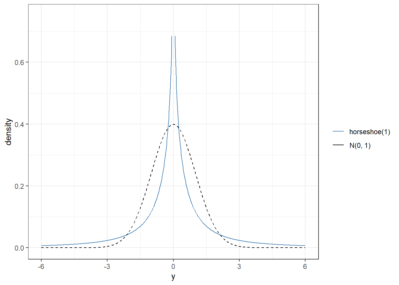

6.3.2 Bayesian logistic regression model (COPE example revisit)

• Data come from a cross-sectional study of 1,225 smokers over the age of 40.

• Each participant was assessed for chronic obstructive pulmonary disease (COPD), and characteristics of the type of cigarette they most frequently smoke were recorded.

• The objective of the study was to identify associations between COPD diagnosis and cigarette characteristics

We will use the following variables from this data set:

• NIC: Nicotine content, in mg

• TAR: Tar content, in mg

• LEN: Length of cigarette, in mm

• copd: 1 = COPD diagnosis, 0 = no COPD diagnosis

NIC	TAR	LEN	copd
0.2	3	68	0
0.3	5	68	0
0.8	14	83	0
0.9	15	83	0
0.8	11	83	0
0.9	15	84	0

• We fit a simple logistic regression, predicting the risk of copd by all covariates as well as all interaction effects

fit4.1 <- brm(copd ~ (.)^2, 
               data = copd, 
               family = bernoulli(link = "logit"), 
               prior = c(
                 prior(normal(0,10), class = "Intercept"),
                 # Prior guess of 25% of the terms are non-zero
                 prior(horseshoe(par_ratio = 2 / 8), class = "b")),
            iter = 7500,
            warmup = 5000,
            chains = 4,
            cores = 5, 
            seed = 123, 
            silent = 2, 
            refresh = 0)

fit4.2 <- brm(copd ~ (.)^2, 
               data = copd, 
               family = bernoulli(link = "logit"), 
               prior = c(
                 prior(normal(0,10), class = "Intercept"),
                 prior(normal(0,10), class = "b")),
            iter = 7500,
            warmup = 5000,
            chains = 4,
            cores = 5, 
            seed = 123, 
            silent = 2, 
            refresh = 0)
# saveRDS(fit4.1, file="data/chap7_h_example4.1")
# saveRDS(fit4.2, file="data/chap7_h_example4.2")

fit4.1 <- readRDS("data/chap7_h_example4.1")
fit4.2 <- readRDS("data/chap7_h_example4.2")

summary(fit4.2)

##  Family: bernoulli 
##   Links: mu = logit 
## Formula: copd ~ (NIC + TAR + LEN)^2 
##    Data: copd (Number of observations: 1225) 
##   Draws: 4 chains, each with iter = 7500; warmup = 5000; thin = 1;
##          total post-warmup draws = 10000
## 
## Population-Level Effects: 
##           Estimate Est.Error l-95% CI u-95% CI Rhat Bulk_ESS Tail_ESS
## Intercept    -5.16      3.30   -11.73     1.20 1.00     4766     4352
## NIC           5.63      6.27    -6.59    18.02 1.00     2652     3835
## TAR          -0.31      0.46    -1.20     0.58 1.00     2669     4452
## LEN           0.02      0.03    -0.04     0.09 1.00     5107     4676
## NIC:TAR       0.06      0.04    -0.02     0.15 1.00     6022     6298
## NIC:LEN      -0.06      0.07    -0.21     0.08 1.00     2631     4007
## TAR:LEN       0.00      0.01    -0.01     0.01 1.00     2644     4475
## 
## Draws were sampled using sampling(NUTS). For each parameter, Bulk_ESS
## and Tail_ESS are effective sample size measures, and Rhat is the potential
## scale reduction factor on split chains (at convergence, Rhat = 1).

summary(fit4.1)

##  Family: bernoulli 
##   Links: mu = logit 
## Formula: copd ~ (NIC + TAR + LEN)^2 
##    Data: copd (Number of observations: 1225) 
##   Draws: 4 chains, each with iter = 7500; warmup = 5000; thin = 1;
##          total post-warmup draws = 10000
## 
## Population-Level Effects: 
##           Estimate Est.Error l-95% CI u-95% CI Rhat Bulk_ESS Tail_ESS
## Intercept    -3.25      0.57    -4.36    -2.07 1.00     6318     5700
## NIC           0.01      0.12    -0.04     0.10 1.00     4425     3544
## TAR           0.00      0.02    -0.03     0.05 1.00     4743     4868
## LEN          -0.00      0.01    -0.01     0.01 1.00     4978     5215
## NIC:TAR       0.02      0.02    -0.00     0.08 1.00     3152     4269
## NIC:LEN       0.00      0.01    -0.00     0.02 1.00     4716     5852
## TAR:LEN       0.00      0.00    -0.00     0.00 1.00     5359     7601
## 
## Draws were sampled using sampling(NUTS). For each parameter, Bulk_ESS
## and Tail_ESS are effective sample size measures, and Rhat is the potential
## scale reduction factor on split chains (at convergence, Rhat = 1).

• An arbitrary cutoff is to select only coefficients with posterior means larger than .02, in which case only NIC and TAR and their interaction were supported by the data.

R Session information

## R version 4.1.3 (2022-03-10)
## Platform: x86_64-w64-mingw32/x64 (64-bit)
## Running under: Windows 10 x64 (build 19044)
## 
## Matrix products: 
## 
## locale:
## [1] LC_COLLATE=English_Canada.1252  LC_CTYPE=English_Canada.1252   
## [3] LC_MONETARY=English_Canada.1252 LC_NUMERIC=C                   
## [5] LC_TIME=English_Canada.1252    
## 
## attached base packages:
## [1] grid      stats     graphics  grDevices utils     datasets  methods  
## [8] base     
## 
## other attached packages:
##  [1] DT_0.22             gtsummary_1.5.2     invgamma_1.1       
##  [4] extraDistr_1.9.1    MCMCpack_1.6-1      MASS_7.3-55        
##  [7] coda_0.19-4         SHELF_1.8.0         bayesplot_1.9.0    
## [10] ggmcmc_1.5.1.1      tidyr_1.2.0         ggpubr_0.4.0       
## [13] tweenr_1.0.2        gganimate_1.0.7     VennDiagram_1.7.1  
## [16] futile.logger_1.4.3 truncnorm_1.0-8     brms_2.16.3        
## [19] Rcpp_1.0.8.3        dplyr_1.0.8         ggplot2_3.3.5

References

Bürkner, Paul-Christian. 2017. “Advanced Bayesian Multilevel Modeling with the r Package Brms.” arXiv Preprint arXiv:1705.11123.

Geweke, John F et al. 1991. “Evaluating the Accuracy of Sampling-Based Approaches to the Calculation of Posterior Moments.” Federal Reserve Bank of Minneapolis.

Lewandowski, Daniel, Dorota Kurowicka, and Harry Joe. 2009. “Generating Random Correlation Matrices Based on Vines and Extended Onion Method.” Journal of Multivariate Analysis 100 (9): 1989–2001.

McElreath, Richard. 2018. Statistical Rethinking: A Bayesian Course with Examples in r and Stan. Chapman; Hall/CRC.

Nakagawa, Shinichi, Paul CD Johnson, and Holger Schielzeth. 2017. “The Coefficient of Determination r 2 and Intra-Class Correlation Coefficient from Generalized Linear Mixed-Effects Models Revisited and Expanded.” Journal of the Royal Society Interface 14 (134): 20170213.

Price, Catherine J, Carole A Kimmel, Rochelle W Tyl, and Melissa C Marr. 1985. “The Developmental Toxicity of Ethylene Glycol in Rats and Mice.” Toxicology and Applied Pharmacology 81 (1): 113–27.

Student. 1908. “The Probable Error of a Mean.” Biometrika, 1–25.

Vehtari, Aki, Andrew Gelman, and Jonah Gabry. 2017. “Practical Bayesian Model Evaluation Using Leave-One-Out Cross-Validation and WAIC.” Statistics and Computing 27 (5): 1413–32.

Watanabe, Sumio, and Manfred Opper. 2010. “Asymptotic Equivalence of Bayes Cross Validation and Widely Applicable Information Criterion in Singular Learning Theory.” Journal of Machine Learning Research 11 (12).