library(tidyverse)
library(gtsummary)
library(DT)

options(scipen = 999)

indo <- read.csv("indo.csv", header = TRUE,fileEncoding="UTF-8-BOM")

# look at new data;
datatable(indo, rownames = FALSE) Heterogeneous Treatment Effects (HTE)
1. Hands-on excerise carrying out a simple risk-based HTE analysis
1.1 Data
Indomethacin for the Prevention of Post-ERCP Pancreatitis Dataset Description Document
This data set is provided by B. Joseph Elmunzer, the primary author of a study published on 2012 in the New England Journal of Medicine, volume 366, pages 1414-1422.
This RCT data contains baseline characteristics and outcomes for 602 participants at increased risk of post-ERCP pancreatitis at 4 centers.
We will be using a modified version of this data
1.2 Fitting a outcome logistic regression without treatment
- Calculate risk score and risk groups
model <- glm(outcome ~ ., data = indo[, c(-1, -2)], family = binomial)

summary(model)
Call:
glm(formula = outcome ~ ., family = binomial, data = indo[, c(-1,
    -2)])

Coefficients:
             Estimate Std. Error z value Pr(>|z|)
(Intercept) -3.717127   1.014570  -3.664 0.000249 ***
age          0.002292   0.011126   0.206 0.836758
risk         0.998877   0.447973   2.230 0.025763 *
gender       0.104782   0.359077   0.292 0.770432
sod         -0.622085   0.508628  -1.223 0.221305
pep          0.077874   0.526669   0.148 0.882452
recpanc     -0.457586   0.358885  -1.275 0.202303
psphinc     -0.330524   0.533223  -0.620 0.535349
precut      -0.898827   0.672453  -1.337 0.181340
difcan      -0.741625   0.513565  -1.444 0.148719
paninj      -0.122011   0.446974  -0.273 0.784875
asa         -0.025352   0.501523  -0.051 0.959684
sodsom      -0.552573   0.357454  -1.546 0.122139
bsphinc      0.178201   0.288961   0.617 0.537435
bstent       0.015613   0.542894   0.029 0.977057
chole        0.932204   0.558188   1.670 0.094908 .
train        0.608712   0.265496   2.293 0.021863 *
---
Signif. codes:  0 '***' 0.001 '**' 0.01 '*' 0.05 '.' 0.1 ' ' 1

(Dispersion parameter for binomial family taken to be 1)

    Null deviance: 467.73  on 600  degrees of freedom
Residual deviance: 437.13  on 584  degrees of freedom
AIC: 471.13

Number of Fisher Scoring iterations: 5
# Calculate predicted risk score;
logOR <- model.matrix(model) %*% coef(model)
logOR_mean <- sum(coef(model)*model$means)
risk_score <- logOR - logOR_mean # centred PI;
indo$risk_score <- risk_score
# Rank patients by risk score and group into Quintile;
indo$riskgp <- cut(
indo$risk_score,
breaks = quantile(indo$risk_score, probs = seq(0, 1, by = 0.2)),
include.lowest = TRUE,
labels = 1:5
)1.3 Fitting a outcome logistic regression with treatment and risk group
trtmodel <- glm(outcome ~ rx*riskgp, data = indo, family = binomial)

summary(trtmodel)
Call:
glm(formula = outcome ~ rx * riskgp, family = binomial, data = indo)

Coefficients:
            Estimate Std. Error z value    Pr(>|z|)
(Intercept)  -2.9957     0.5916  -5.064 0.000000411 ***
rx           -1.0473     1.1693  -0.896    0.370413
riskgp2       0.9480     0.7008   1.353    0.176125
riskgp3       1.1350     0.7177   1.581    0.113779
riskgp4       1.7636     0.6650   2.652    0.008004 **
riskgp5       2.3026     0.6519   3.532    0.000412 ***
rx:riskgp2    0.6527     1.3342   0.489    0.624712
rx:riskgp3    0.3744     1.3222   0.283    0.777062
rx:riskgp4    0.1200     1.2827   0.094    0.925479
rx:riskgp5    0.2465     1.2464   0.198    0.843200
---
Signif. codes:  0 '***' 0.001 '**' 0.01 '*' 0.05 '.' 0.1 ' ' 1

(Dispersion parameter for binomial family taken to be 1)

    Null deviance: 467.73  on 600  degrees of freedom
Residual deviance: 427.03  on 591  degrees of freedom
AIC: 447.03

Number of Fisher Scoring iterations: 6
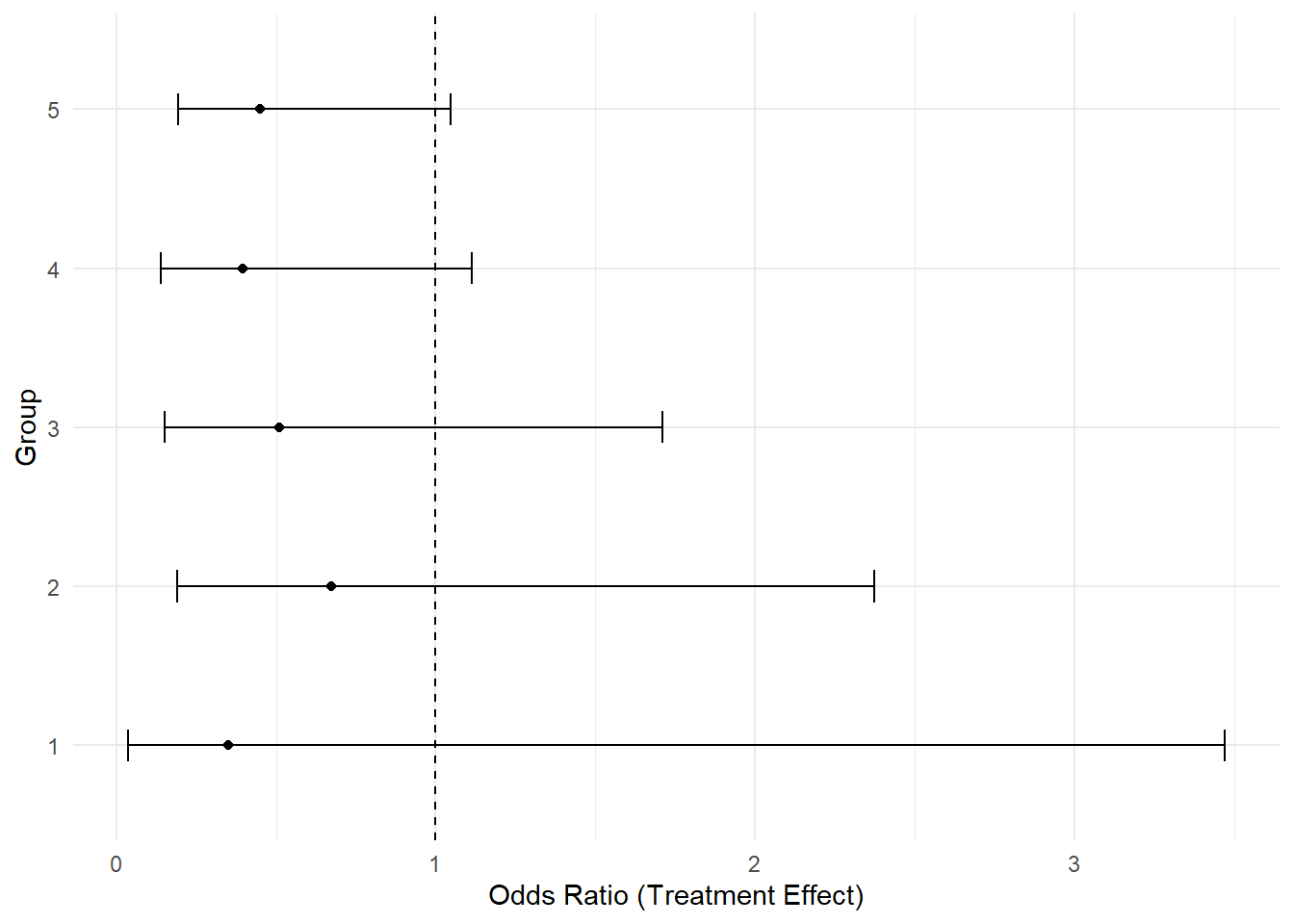
# Calculate risk group-specific treatment effect on the OR scale;
# Extract coefficients and variance-covariance matrix
coefficients <- coef(trtmodel)
vcov_matrix <- vcov(trtmodel)
# Initialize a data frame to store results
results <- data.frame(
riskgp = levels(indo$riskgp),
logOR = NA,
SE = NA,
OR = NA,
lower_CI = NA,
upper_CI = NA
)
# Loop through each group
for (i in 1:length(levels(indo$riskgp))) {
grp <- levels(indo$riskgp)[i]
# Create a contrast vector
contrast <- rep(0, length(coefficients))
names(contrast) <- names(coefficients)
# Main effect of rx
contrast["rx"] <- 1
# Add interaction term if not the reference group
if (grp != levels(indo$riskgp)[1]) {
interaction_term <- paste0("rx:riskgp", grp)
contrast[interaction_term] <- 1
}
# Compute the log odds ratio
logOR <- sum(contrast * coefficients)
# Compute the standard error
SE <- sqrt(t(contrast) %*% vcov_matrix %*% contrast)
# Compute the odds ratio and confidence intervals
OR <- exp(logOR)
lower_CI <- exp(logOR - 1.96 * SE)
upper_CI <- exp(logOR + 1.96 * SE)
# Store the results
results$logOR[i] <- logOR
results$SE[i] <- SE
results$OR[i] <- OR
results$lower_CI[i] <- lower_CI
results$upper_CI[i] <- upper_CI
}
# Plot the group-specific rx effects
ggplot(results, aes(x = OR, y = riskgp)) +
geom_point() +
geom_errorbarh(aes(xmin = lower_CI, xmax = upper_CI), height = 0.2) +
geom_vline(xintercept = 1, linetype = "dashed") +
xlab("Odds Ratio (Treatment Effect)") +
ylab("Group") +
theme_minimal()
2. Hands-on excerise to run a causal forest
2.1 Prognostic Model (Random Forest)
library(randomForest)
rf_model <- randomForest(outcome ~ ., data = indo[, c(-1, -2)])
indo$rf_prob <- predict(rf_model, type = "response")
2.2 Fit Causal Forest Model
# library(devtools)
# install_github("susanathey/causalTree")
library(causalTree)
cf_model <- causalForest(
  formula = outcome ~ rx + rf_prob + age + risk + gender + sod + pep + recpanc + psphinc + precut + difcan + paninj + asa + sodsom + bsphinc + bstent + chole + train,
  data = indo,
  treatment = indo$rx,
  ncov_sample = 10,
  ncolx = 18,
  split.Rule = "CT",
  cv.option = "CT",
  split.Honest = TRUE,
  cv.Honest = TRUE,
  split.Bucket = FALSE,
  bucketNum = 5,
  bucketMax = 100,
  minsize = 20
)

indo$cARD <- predict(cf_model, newdata=indo)
# Rank patients by treatment effect and group into quintile;
indo$cARDgp <- cut(
indo$cARD,
breaks = quantile(indo$cARD, probs = seq(0, 1, by = 0.2)),
include.lowest = TRUE,
labels = 1:5
)
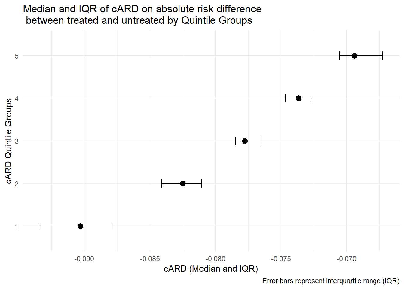
# calculate mean and IQR of CARD for each group and plot it.
cARD_summary <- indo %>%
group_by(cARDgp) %>%
summarize(
median_cARD = median(cARD, na.rm = TRUE),
IQR_lower = quantile(cARD, 0.25, na.rm = TRUE),
IQR_upper = quantile(cARD, 0.75, na.rm = TRUE),
.groups = "drop"
)
print(cARD_summary)# A tibble: 5 × 4
cARDgp median_cARD IQR_lower IQR_upper
<fct> <dbl> <dbl> <dbl>
1 1 -0.0877 -0.0909 -0.0855
2 2 -0.0811 -0.0829 -0.0800
3 3 -0.0772 -0.0780 -0.0762
4 4 -0.0730 -0.0741 -0.0717
5 5 -0.0671 -0.0690 -0.0653# plot treatment effect by effect groups;
ggplot(cARD_summary, aes(y = cARDgp, x = median_cARD)) +
geom_point(size = 3) +
geom_errorbarh(aes(xmin = IQR_lower, xmax = IQR_upper), height = 0.2) +
theme_minimal() +
labs(
title = "Median and IQR of cARD on absolute risk difference \n between treated and untreated by Quintile Groups",
y = "cARD Quintile Groups",
x = "cARD (Median and IQR)",
caption = "Error bars represent interquartile range (IQR)"
)
