Predictive modelling lab1

1. Hands-on excerise building a simple predictive logsitic regression model

1.1 Descriptive analysis

• For this tutorial, we will be using the OVA data. This data set contains information on the follow-up of patients with severe ovary cancer.

• We use SURV, survival status at 4 years as a binary outcome

• Predictors considered are: KARN, BRODERS, FIGO, ASCITES, DIAM, AGE, and RACE

• The data are as follows:

  • T survival time in days
  • D 1 = dead at time T; 0 = alive at time T
  • SURV 1 = T > 1460 (4 years); 0 = T <= 1460
  • KARN Karnovsky-index, coded as 6 ( <= 60), 7, 8, 9, 10 (= 100)
  • BRODERS Broders grading
  • FIGO 3 or 4
  • ASCITES 1 = absent; 2 = present; 0 = unknown
  • DIAM diameter residual tumor 3 = >= 5 cm; 4 = 2 - 5 cm; 5 = 1 - 2 cm; 6 = < 1 cm; 7 = only microscopical residuals
  • AGE age at diagnose (year)
  • Race = 1 white, 0 = non-white;

library(tidyverse)
library(gtsummary)
library(DT)

ova <- read.csv("OVA.csv", header = TRUE)
ova$race <- as.factor(ova$race)

# look at new data;
datatable(ova,
          rownames = FALSE,
          options = list(dom = 't')) 

# display summary statistics by survival status;
ova %>% 
  tbl_summary(
  by = surv,
  missing_text = "(Missing)") %>%
  add_overall() %>%
  add_p()

Characteristic	Overall N = 3581	0 N = 2461	1 N = 1121	p-value2
t	735 (369, 1,620)	478 (237, 779)	1,891 (1,667, 2,159)	<0.001
d	266 (74%)	246 (100%)	20 (18%)	<0.001
karn				0.003
6	20 (5.6%)	19 (7.7%)	1 (0.9%)
7	46 (13%)	39 (16%)	7 (6.3%)
8	47 (13%)	34 (14%)	13 (12%)
9	108 (30%)	67 (27%)	41 (37%)
10	137 (38%)	87 (35%)	50 (45%)
broders				0.004
1	42 (14%)	19 (9.2%)	23 (23%)
2	89 (29%)	63 (31%)	26 (26%)
3	127 (41%)	94 (46%)	33 (33%)
4	49 (16%)	30 (15%)	19 (19%)
(Missing)	51	40	11
figo				<0.001
3	262 (73%)	164 (67%)	98 (88%)
4	96 (27%)	82 (33%)	14 (13%)
ascites				0.005
0	52 (15%)	38 (15%)	14 (13%)
1	94 (26%)	52 (21%)	42 (38%)
2	212 (59%)	156 (63%)	56 (50%)
diam				<0.001
3	145 (41%)	119 (48%)	26 (23%)
4	68 (19%)	49 (20%)	19 (17%)
5	49 (14%)	33 (13%)	16 (14%)
6	67 (19%)	35 (14%)	32 (29%)
7	29 (8.1%)	10 (4.1%)	19 (17%)
age	55 (45, 65)	58 (50, 66)	49 (40, 56)	<0.001
race				0.003
non-white	136 (38%)	81 (33%)	55 (49%)
white	222 (62%)	165 (67%)	57 (51%)
1 Median (Q1, Q3); n (%)
2 Wilcoxon rank sum test; Pearson’s Chi-squared test

1.2 Data manipulation

• We will have a guest lecture on missing data by Prof. Aya Mitani, see course schedule.
• We can use multiple imputation to handle missing data, this will be covered in the guest lecture.
• In this example, we show how you can summarize missingness by other covariates and we create a new category for unkown BRODERS scores (0=unknown)

#step 1: summarize data by missing status;
# any variables have differential distribution by missing broder scores?;
ova %>%
  mutate(missing = ifelse(is.na(broders)==T,1,0)) %>% 
  select(-broders) %>%
  tbl_summary(
  by = missing,
  missing_text = "(Missing)") %>%
  add_p()

Characteristic	0 N = 3071	1 N = 511	p-value2
t	779 (385, 1,668)	649 (226, 1,421)	0.043
d	225 (73%)	41 (80%)	0.3
surv	101 (33%)	11 (22%)	0.11
karn			0.7
6	17 (5.5%)	3 (5.9%)
7	37 (12%)	9 (18%)
8	40 (13%)	7 (14%)
9	96 (31%)	12 (24%)
10	117 (38%)	20 (39%)
figo			0.069
3	230 (75%)	32 (63%)
4	77 (25%)	19 (37%)
ascites			0.4
0	42 (14%)	10 (20%)
1	84 (27%)	10 (20%)
2	181 (59%)	31 (61%)
diam			0.3
3	123 (40%)	22 (43%)
4	60 (20%)	8 (16%)
5	39 (13%)	10 (20%)
6	57 (19%)	10 (20%)
7	28 (9.1%)	1 (2.0%)
age	56 (46, 65)	54 (45, 66)	>0.9
race			0.4
non-white	114 (37%)	22 (43%)
white	193 (63%)	29 (57%)
1 Median (Q1, Q3); n (%)
2 Wilcoxon rank sum test; Pearson’s Chi-squared test; Fisher’s exact test

#Step 2: try simple imputation, we replace missing value with mean;
ova <- ova %>%
  mutate(broders2 = ifelse(is.na(broders)==T,mean(broders, na.rm = T),broders)) #if missing assign mean value, otherwise assign the original value;

Tips on handling missing data

• when you have multiple variables with missing information, you can use data vistualization to display missing pattern, reference tutorial R see, https://cran.r-project.org/web/packages/naniar/vignettes/naniar-visualisation.html

• Under missing at random, Rule of thumb, if you have <= 25% missing, you can consider multiple imputation. Number of imputed copies to be considered between 5 to 20.

• For categorical variable, adding a new category for missing can be preferred if you don’t want to make any missing assumptions.

• At this step, you can also evaluate your data and see if recoding is needed to collapse categories (categories with rare outcome or categories with small cell).

1.3 Model building strategies

• Predictive models should include those variables that reflect the study population of interest

• When more is not better: variables can be highly correlated, removing one of the highly correlated predictor does not compromise the model performance and the reduced model is computationally more efficient.

• Good practice to assess pair-wise correlation before building your predictive model

• You can also use model selection approaches for example, LASSO or bootstrap + stepwise (not stepwise by itself), however, since we are building a predictive model. Model selection should ideally be performed to maximize predictive power and accuracy not fit! That is comparing predictive model based on C-statistics, ROC not AIC or BIC.

#create a dataset to host all variables that will be used to build the prediction model;
ova2 <- ova %>% select(-t, -d, -broders)

• now let’s build a model no interaction and no non-linear terms, just a simple additive logistic regression model

m0 <- glm(surv ~ as.factor(karn)+as.factor(figo)+as.factor(ascites)+as.factor(diam)+age+as.factor(broders2)+ as.factor(race), family="binomial", data = ova2)
summary(m0)

Call:
glm(formula = surv ~ as.factor(karn) + as.factor(figo) + as.factor(ascites) + 
    as.factor(diam) + age + as.factor(broders2) + as.factor(race), 
    family = "binomial", data = ova2)

Coefficients:
                                    Estimate Std. Error z value Pr(>|z|)    
(Intercept)                          0.58684    1.24681   0.471 0.637876    
as.factor(karn)7                     1.07070    1.14943   0.932 0.351591    
as.factor(karn)8                     1.89273    1.12228   1.687 0.091698 .  
as.factor(karn)9                     1.81644    1.09084   1.665 0.095876 .  
as.factor(karn)10                    1.71248    1.08840   1.573 0.115629    
as.factor(figo)4                    -0.91114    0.35547  -2.563 0.010371 *  
as.factor(ascites)1                 -0.01091    0.43835  -0.025 0.980147    
as.factor(ascites)2                 -0.41064    0.39867  -1.030 0.303002    
as.factor(diam)4                     0.54884    0.38125   1.440 0.149981    
as.factor(diam)5                     0.69043    0.42123   1.639 0.101192    
as.factor(diam)6                     1.22101    0.37354   3.269 0.001080 ** 
as.factor(diam)7                     1.70216    0.49674   3.427 0.000611 ***
age                                 -0.04090    0.01033  -3.961 7.48e-05 ***
as.factor(broders2)2                -1.00286    0.45200  -2.219 0.026505 *  
as.factor(broders2)2.59609120521173 -1.25667    0.52676  -2.386 0.017050 *  
as.factor(broders2)3                -1.18499    0.42873  -2.764 0.005711 ** 
as.factor(broders2)4                -0.37914    0.50507  -0.751 0.452856    
as.factor(race)white                -0.26649    0.28245  -0.944 0.345424    
---
Signif. codes:  0 '***' 0.001 '**' 0.01 '*' 0.05 '.' 0.1 ' ' 1

(Dispersion parameter for binomial family taken to be 1)

    Null deviance: 444.89  on 357  degrees of freedom
Residual deviance: 350.71  on 340  degrees of freedom
AIC: 386.71

Number of Fisher Scoring iterations: 5

1.4 Model performance

• Two key elements in assessing the performance of a fitted logistic regression model are the assessment of model calibration and model discrimination.

• Calibration refers to the agreement between observed outcomes and predictions (brier score, calibration plot)

• Discrimination refers to the ability of model predictions to discriminate between those with and those without the outcome (C-statistics, ROC)

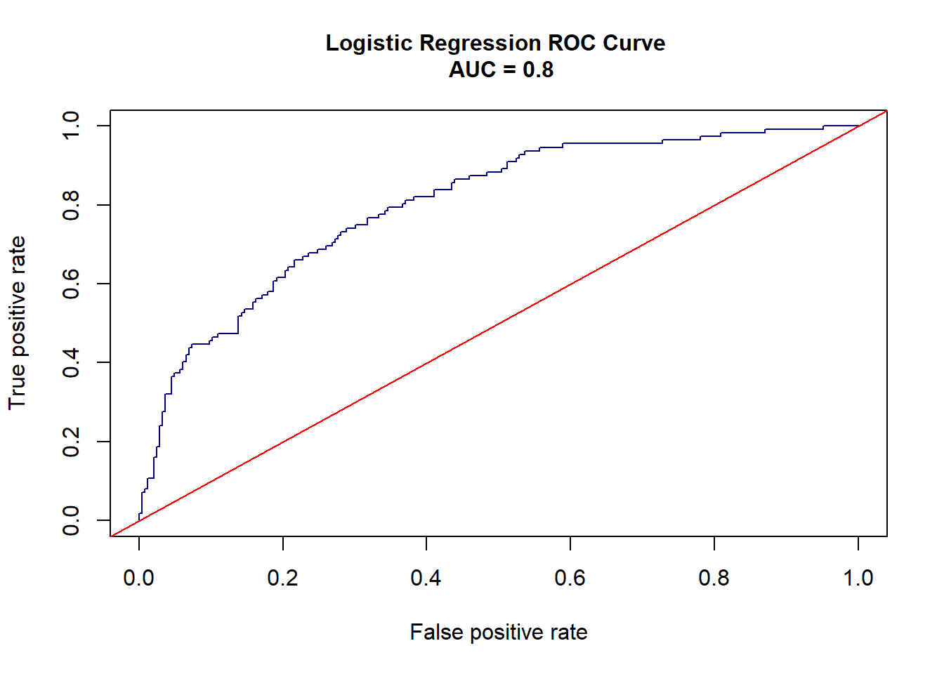
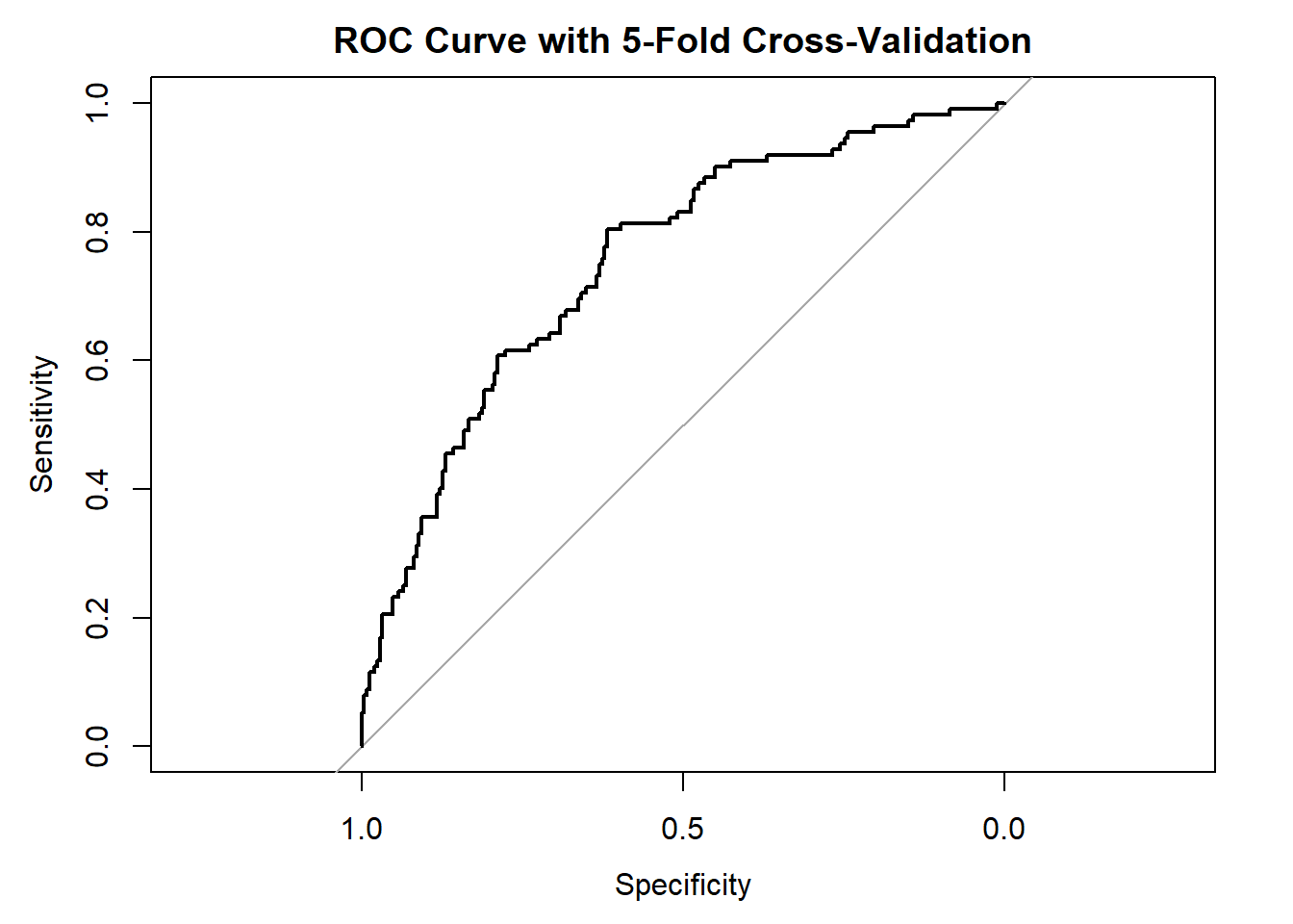
• First, lets estimate c-statistics (AUC) and plot ROC curve

  • “The c-statistic is defined as the proportion of all possible pairs of subjects, one of whom experienced the outcome of interest and one of whom did not, in which the subject who experienced the outcome of interest had a higher predicted probability of the outcome occurring than does the subject who did not experience the outcome.” - From Austin, Harrell, and Steyerberg, 2021

# install.packages('ROCR')
library(ROCR)

# in-sample: the same training data set on which the model was fit;
prob <- predict.glm(m0, type='response', newdata =  ova2)
pred <- prediction(prob, ova2$surv)

# AUC
auc <- performance(pred,"auc")@y.values[[1]][1]
auc #c-statistics for model m0 is 0.8 pretty good!

[1] 0.8007767

# plot the ROC curve
perf <- performance(pred,"tpr","fpr")
plot(perf, col="navyblue", cex.main=1,
     main= paste("Logistic Regression ROC Curve \n AUC =", round(auc,3)))
abline(a=0, b = 1, col='red')

# we can obtain a confidence interval for AUC via bootstrap;
# package pROC has a function that allows you do do this more easily;
# I provided below sample codes to do bootstrap manually;

n<-dim(ova2)[1]
auc.boot <- rep(NA, 1000) #initiating a empty vector of size 1000 to save the bootstrap auc;

set.seed(123)
for(i in 1:1000){
  # random draw with replacement to form a bootstrap sample with same size as the original data;
    obs.boot <- sample(x = 1:n, size = n, replace = T)
    data.boot <- ova2[obs.boot, ]
    
    # fit the model on bootstrap sample
    m0.boot <- glm(m0$formula , #extracting model formula from m0;
                      data=data.boot,
                      family = binomial(link = "logit"))
    
    # calculate and save auc for each bootstrap iteration;
    prob1 = predict(m0.boot, type='response', data.boot)
    pred1 = prediction(prob1, data.boot$surv)
    auc.boot[i] <- performance(pred1,"auc")@y.values[[1]][1]
}

# 95% CI for auc using empirical distribution;
quantile(auc.boot, c(.025, .975)) 

     2.5%     97.5% 
0.7777468 0.8647307 

• Brier score is simply the mean of squared differences between the predicted probability of outcome = 1 and the observed event status (0 or 1). A measurement that quantifies the predictive accuracy.

• Brier score between 0 and 1, 0 is perfect prediction; 0.25 is predicting by chance - as flipping a coin; 1 is worst prediction, worst than flipping a coin.

\[ \text{Brier score} = \frac{1}{N} \sum_{i=1}^N (P(y_i=1 \mid x_{i1}, \ldots, x_{ip}) - y_i)^2 \]

BrierScore <- mean((prob-ova2$surv)^2)
BrierScore

[1] 0.1615669

#try this yourself, can you use the bootstrap code to get the empirical distirbution of BrierScore?

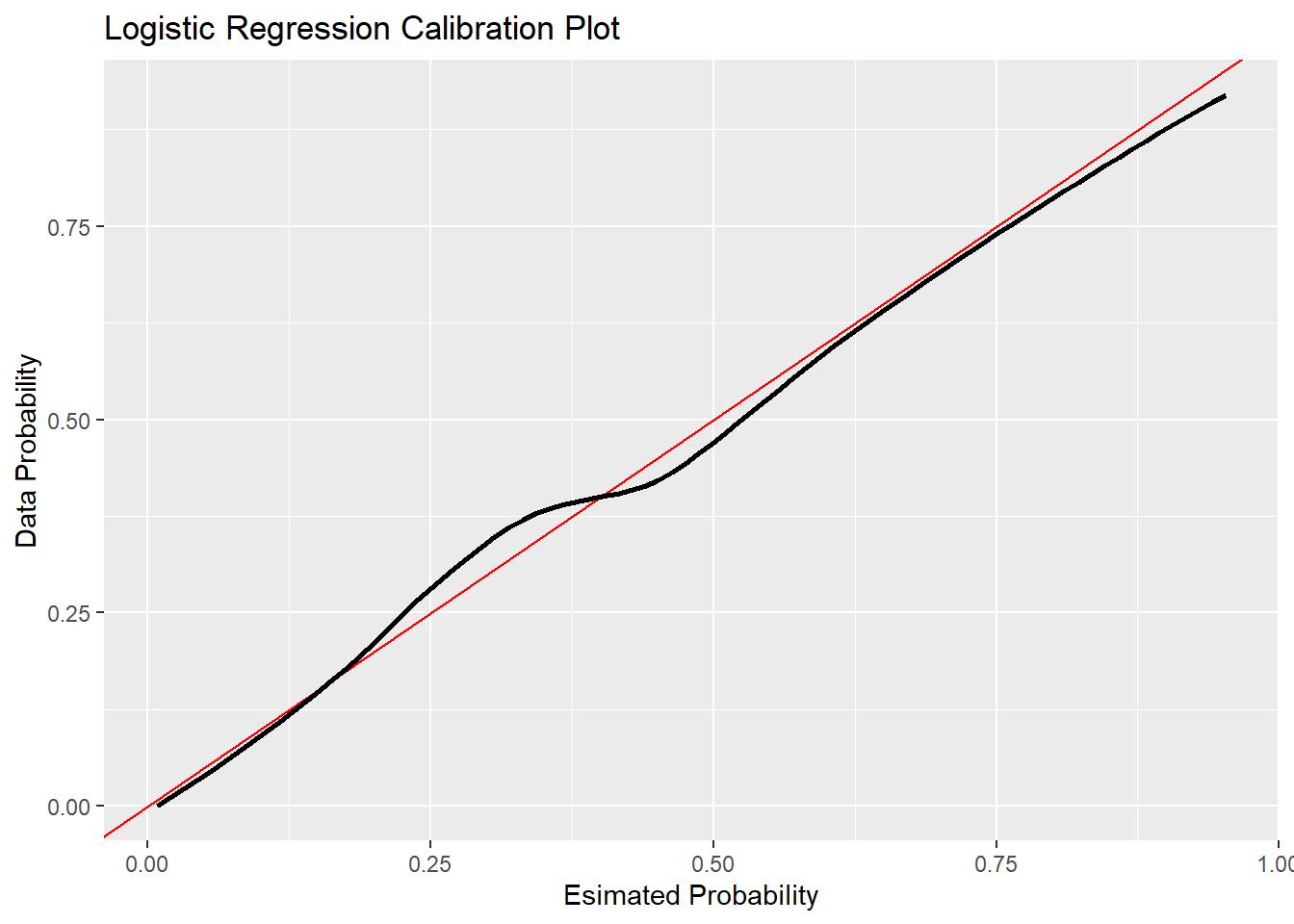
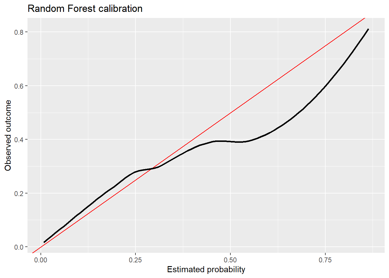
• Regression calibration plot to compare the probability of outcome from the data with the estimated probability of outcome from the model.
  • perfect calibration if the empirical probability matches with the model estimated probability in a diagonal line,
  • we can fit a linear regression model for the data probability (as y) and model estimated probability (as x) and report the intercept and slope of this simple linear regression as the calibration intercept and slope

pdat <- with(ova2, data.frame(surv,prob = predict(m0, type = "response")))

lm(surv ~ prob, data = pdat)

Call:
lm(formula = surv ~ prob, data = pdat)

Coefficients:
(Intercept)         prob  
   0.001826     0.994164  

# intercept estimated at 0.001157 and slope estimated at 0.9963;

ggplot(pdat, aes(prob,surv))+
  geom_abline(slope=1, intercept = 0, color = "red")+
  geom_smooth(method = stats::loess, se = FALSE, color="black")+
  xlab("Esimated Probability")+
  ylab("Data Probability")+
  ggtitle("Logistic Regression Calibration Plot")

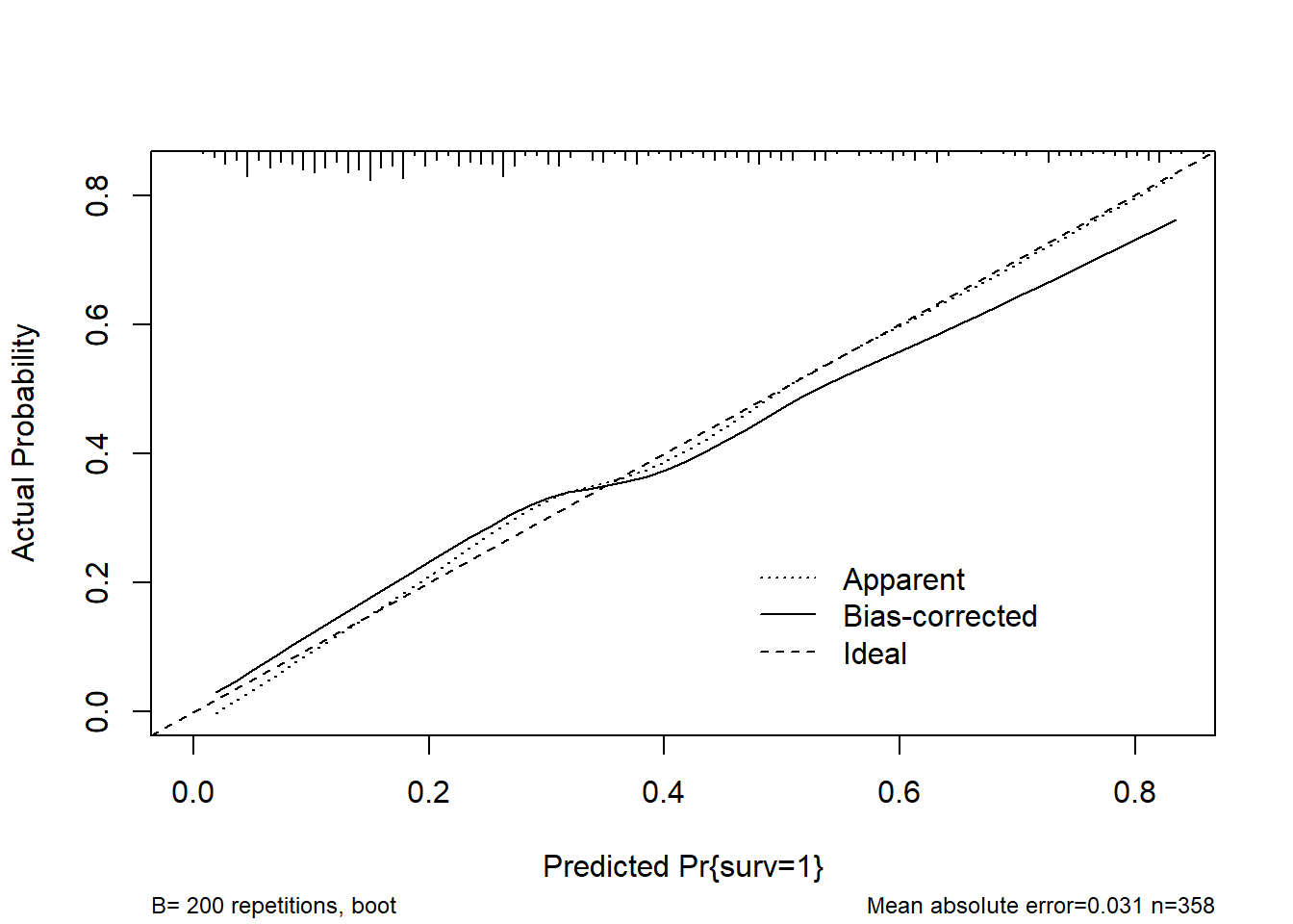
# getting calibration plot using rms package;
library(rms)
ova2 <- ova2 %>%
  mutate(karn = as.factor(karn),
         figo = as.factor(figo),
         ascites = as.factor(ascites),
         diam = as.factor(diam),
         broders2 = as.factor(broders2))

m0_rms <- lrm( surv ~ karn + figo + ascites + diam + age + broders2, data = ova2, x = TRUE, y = TRUE)
plot(calibrate(m0_rms, B=200))

n=358   Mean absolute error=0.031   Mean squared error=0.00115
0.9 Quantile of absolute error=0.055

#Resampling Validation of a Fitted Model using rms package (might have seen this from Biostat 2 with Kevin);
validate(m0_rms, B=200)

          index.orig training    test optimism index.corrected   n
Dxy           0.6007   0.6418  0.5608   0.0811          0.5196 200
R2            0.3225   0.3710  0.2625   0.1085          0.2140 200
Intercept     0.0000   0.0000 -0.1428   0.1428         -0.1428 200
Slope         1.0000   1.0000  0.7451   0.2549          0.7451 200
Emax          0.0000   0.0000  0.0915   0.0915          0.0915 200
D             0.2578   0.3039  0.2042   0.0997          0.1581 200
U            -0.0056  -0.0056  0.0210  -0.0266          0.0210 200
Q             0.2634   0.3095  0.1832   0.1263          0.1371 200
B             0.1619   0.1523  0.1707  -0.0184          0.1803 200
g             1.5101   2.2278  1.5882   0.6396          0.8705 200
gp            0.2571   0.2735  0.2290   0.0445          0.2126 200

• Somers’ Dxy, \(= 2 \times (C-0.5)\), in this case the corrected Dxy = 0.5186, thus the corrected c-statistics/AUC is 0.5186/2 + 0.5 = 0.7593.

1.5 Updating model by adding a non-linear term on variable age and compare this model to the simple additive model

• fitting a new model with a spline term on variable age

• comparing this model to the previous model on prediction performance

library(splines2)

m1 <- glm(surv ~ karn + figo + ascites + diam + splines::ns(age,3) + broders2 + race, family="binomial", data = ova2)
summary(m1)

Call:
glm(formula = surv ~ karn + figo + ascites + diam + splines::ns(age, 
    3) + broders2 + race, family = "binomial", data = ova2)

Coefficients:
                         Estimate Std. Error z value Pr(>|z|)    
(Intercept)              -1.62758    1.49976  -1.085 0.277821    
karn7                     1.14847    1.16256   0.988 0.323210    
karn8                     1.95600    1.13747   1.720 0.085503 .  
karn9                     2.07058    1.10653   1.871 0.061312 .  
karn10                    1.83810    1.10224   1.668 0.095396 .  
figo4                    -0.93518    0.36259  -2.579 0.009903 ** 
ascites1                 -0.06529    0.44834  -0.146 0.884212    
ascites2                 -0.50972    0.41020  -1.243 0.214005    
diam4                     0.45356    0.39147   1.159 0.246613    
diam5                     0.64665    0.42800   1.511 0.130818    
diam6                     1.07618    0.37827   2.845 0.004441 ** 
diam7                     1.65266    0.50196   3.292 0.000993 ***
splines::ns(age, 3)1     -2.62417    0.68841  -3.812 0.000138 ***
splines::ns(age, 3)2      1.40133    2.30289   0.609 0.542851    
splines::ns(age, 3)3     -0.14007    1.32386  -0.106 0.915739    
broders22                -1.00967    0.46016  -2.194 0.028223 *  
broders22.59609120521173 -1.37212    0.54229  -2.530 0.011399 *  
broders23                -1.27183    0.43719  -2.909 0.003625 ** 
broders24                -0.44363    0.51743  -0.857 0.391241    
racewhite                -0.24631    0.28716  -0.858 0.391032    
---
Signif. codes:  0 '***' 0.001 '**' 0.01 '*' 0.05 '.' 0.1 ' ' 1

(Dispersion parameter for binomial family taken to be 1)

    Null deviance: 444.89  on 357  degrees of freedom
Residual deviance: 342.14  on 338  degrees of freedom
AIC: 382.14

Number of Fisher Scoring iterations: 5

prob <- predict.glm(m1, type='response', newdata =  ova2)
pred <- prediction(prob, ova2$surv)

# AUC
auc <- performance(pred,"auc")@y.values[[1]][1]
auc #new auc is 0.812, improved!

[1] 0.8123911

BrierScore <- mean((prob-ova2$surv)^2)
BrierScore #also improved;

[1] 0.1573991

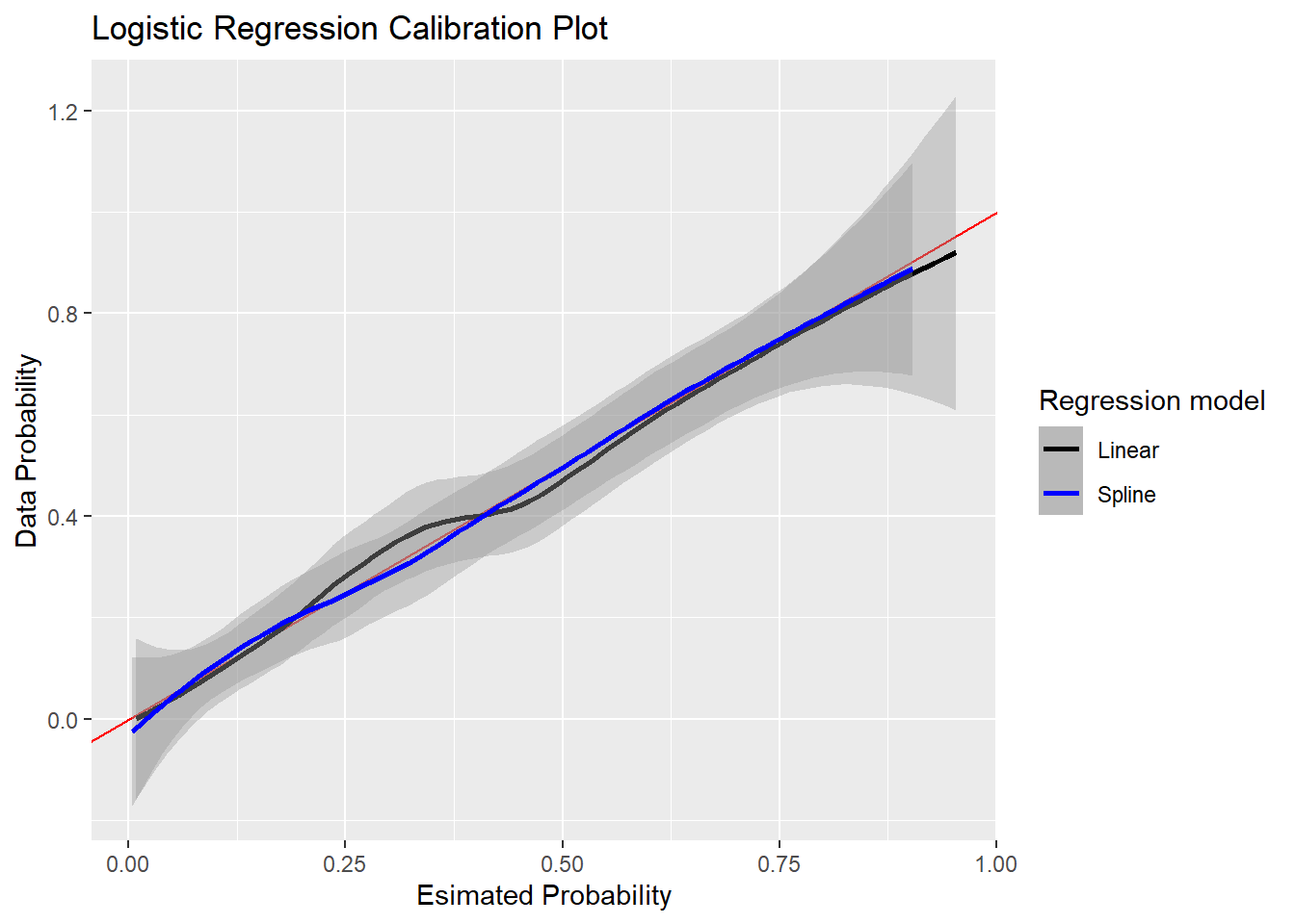
#comparing two calibration plots;
# pdat <- with(ova2, data.frame(surv,prob = predict(m0, type = "response")))
pdat_nonlinear <- with(ova2, data.frame(surv,prob_linear = predict(m0, type = "response"), prob_nonlinear = predict(m1, type = "response")))

ggplot(pdat_nonlinear, aes(prob_linear,surv))+
  geom_abline(slope=1, intercept = 0, aes(colour = "Reference"), colour="red")+
  geom_smooth(aes(x= prob_linear,y=surv,colour = "Linear"), method = stats::loess)+
  geom_smooth(aes(x=prob_nonlinear,y=surv,colour = "Spline"), method = stats::loess)+
  labs(x="Esimated Probability",
       y="Data Probability")+
  scale_color_manual(name="Regression model",
                     breaks=c("Reference","Linear","Spline"),
                     values = c("Reference"="red","Linear"="black","Spline"="blue")) +
  ggtitle("Logistic Regression Calibration Plot")

• The spline model has better predictive performance comparing to the linear model.

2. Special topic with ML-based prediction models

Random Forest

An ensemble classifier that builds many decision trees on bootstrapped samples and averages their predicted probabilities (majority vote for classes). Each split considers a random subset of features, injecting decorrelation among trees.

For binary outcomes, each tree outputs a class probability; the forest prediction is the mean across trees.

Key parameters: - num.trees - mtry (number of features tested per split; \(\sqrt{p}\) is a common default), - min.node.size / max.depth (controls overfitting), - class weights or sample.fraction for imbalance.

Strengths: - Captures nonlinearities and high-order interactions automatically. - Handles mixed data types and is robust to outliers/monotone recodes. - Usually competitive “out of the box” with minimal tuning of the parameters.

Weaknesses: - Less interpretable than a simple logistic model; use permutation importance and partial dependence for explanation. - Correlated predictors can dilute importance across similar variables.

library(ranger)

ova2 <- ova2 %>%
mutate(surv_f = factor(surv, levels = c(0, 1)))

# 70/30 slip cross-validation;
idx_tr <- sample(seq_len(nrow(ova2)), size = floor(0.7 * nrow(ova2)))
train <- ova2[idx_tr, ]
test <- ova2[-idx_tr, ]

pred_vars <- c("karn","figo","ascites","diam","age","broders2","race")
p <- length(pred_vars)                
mtry_val <- max(1, floor(sqrt(p)))     

rf_fit <- ranger(
  formula = as.formula(
    paste("surv_f ~", paste(pred_vars, collapse = " + "))
  ),
  data = train,
  num.trees = 1000,
  mtry = mtry_val,
  min.node.size = 5,
  probability = TRUE,
  importance = "permutation",
  seed = 123
)


rf_prob_test <- predict(rf_fit, test)$predictions[, "1"]


pr <- prediction(rf_prob_test, test$surv)
auc <- performance(pr, "auc")@y.values[[1]][1]
bri <- mean((rf_prob_test - test$surv)^2)

perf <- performance(pr, "tpr", "fpr")
plot(perf,
cex.main = 1,
main = paste0("Random Forest ROC | AUC=", round(auc, 3),
" | Brier=", round(bri, 3)))
abline(a = 0, b = 1, col = "red")

# calibration;
pdat <- tibble(surv = test$surv, prob = rf_prob_test)
ggplot(pdat, aes(prob, surv)) +
geom_abline(slope = 1, intercept = 0, color = "red") +
geom_smooth(method = stats::loess, se = FALSE, color = "black") +
labs(x = "Estimated probability", y = "Observed outcome",
title = "Random Forest calibration")

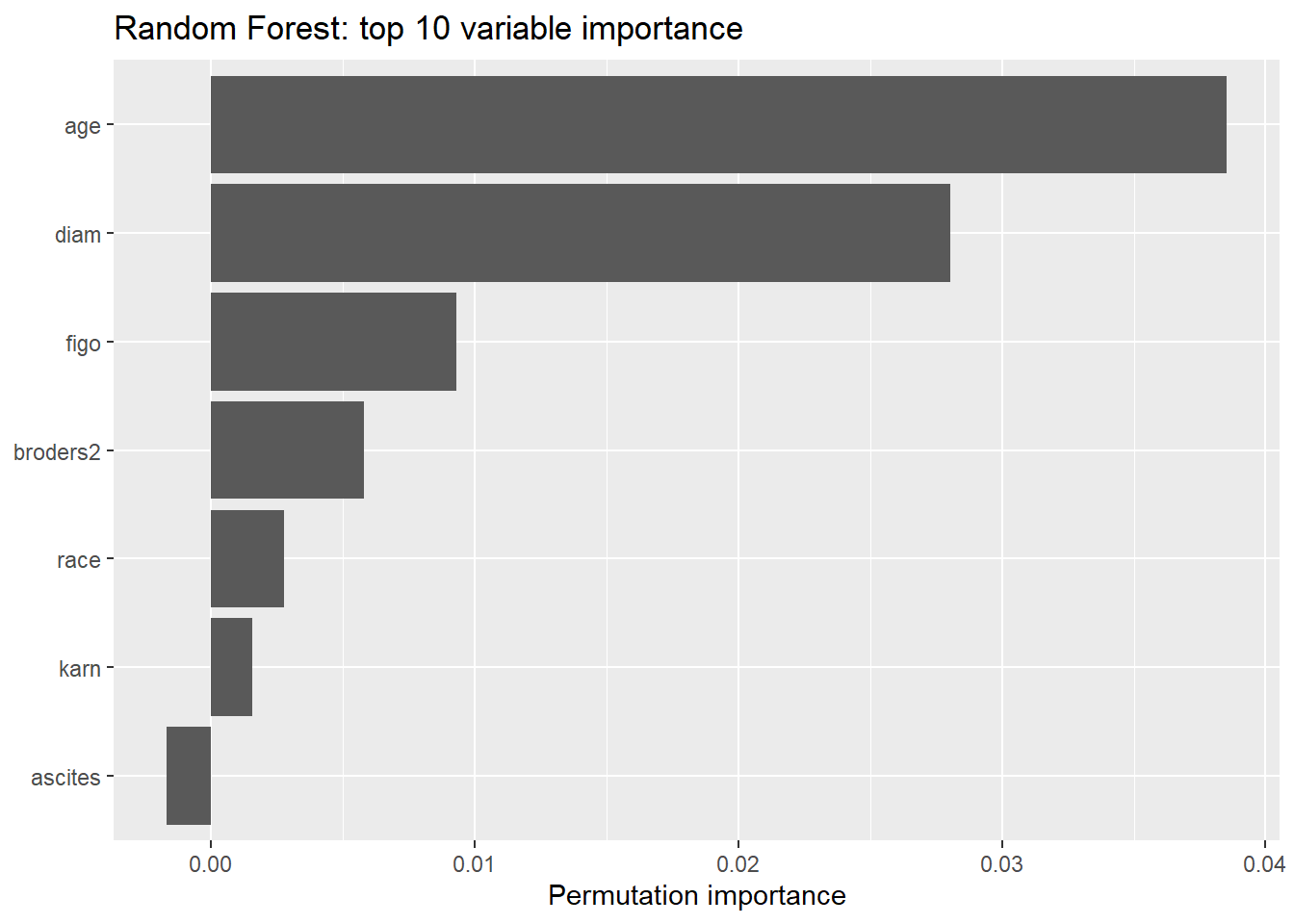
# variable importance;

rf_vi <- enframe(rf_fit$variable.importance,
name = "variable", value = "importance") %>%
arrange(desc(importance))

rf_vi %>% slice_head(n = 10)

# A tibble: 7 × 2
  variable importance
  <chr>         <dbl>
1 age         0.0385 
2 diam        0.0281 
3 figo        0.00930
4 broders2    0.00579
5 race        0.00278
6 karn        0.00155
7 ascites    -0.00168

rf_vi %>%
slice_max(order_by = importance, n = 10) %>%
ggplot(aes(x = reorder(variable, importance), y = importance)) +
geom_col() +
coord_flip() +
labs(x = NULL, y = "Permutation importance",
title = "Random Forest: top 10 variable importance")

# comparing with logistic regression;

prob_m1_test <- predict(m1, type = "response", newdata = test)
pr_m1 <- prediction(prob_m1_test, test$surv)
auc_m1 <- performance(pr_m1, "auc")@y.values[[1]][1]
bri_m1 <- mean((prob_m1_test - test$surv)^2)

tibble(
Model = c("Random Forest", "Logistic (spline)"),
AUC = c(auc, auc_m1),
Brier = c(bri, bri_m1)
) %>% arrange(desc(AUC))

# A tibble: 2 × 3
  Model               AUC Brier
  <chr>             <dbl> <dbl>
1 Logistic (spline) 0.777 0.152
2 Random Forest     0.702 0.178