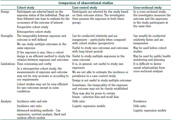
Reviewing of common observational study designs and reporting of observational study
Reviewing survival analysis (Biostatistics II)
About me
I am an Assistant Professor in Health Services Research (outcomes and evaluation method emphasis) at IHPME. I also hold a cross-appointment at the Division of Biostatistics.
My primary research focuses on developing methodology for statistical inference with complex longitudinal data in comparative effectiveness research. My areas of methodological interest include causal inference, Bayesian statistics, longitudinal data analysis, bias analysis, and mixture and joint modelling. If you are interested in working with me for your research/thesis projects, feel free to reach me.
Introducing Yourself
You can share your program, research interests, learning goals, and hobby.
Syllabus
Detailed course syllabus is posted on Quercus.
Important Notes
Course schedule
Course materials
The lecture notes will be the main resource for this course.
All course notes (or link to notes) will be posted on Quercus. Notes for certain sessions will be open-acess and hosted on this website, https://kuan-liu.github.io/biostat3/.
Additional reading materials (e.g., articles) will be posted on Quercus
Example R scripts/ R markdown files and data will be uploaded to Quercus.
R and RStudio
We will be primarily using R via RStudio for this course!
You are encouraged to write your individual assignment using Quarto or Rmarkdown.
Please bring your laptop to sessions on the course calendar that flagged with R in description.
‘Grading’
Participation/attendance
Three group presentations for each lecture block (10% x 3 = 30%).
A team of 2 to 3 students for give a 10 mins presentation followed by 3 mins Q&A. I suggest collaborating with different peers for each group presentation. I am happy to facility random grouping if preferred.
Three individual assignments for each lecture block (10% x 3 = 30%).
One group course report (40%). Instruction will be handed out and submitted on Quercus.
Can I work with peers for individual assignments?
Auditing the course
Welcome but with caveats (past experience from other courses)
seriously committed (try not to miss classes)
expected to have the same level of participation in in-class activities
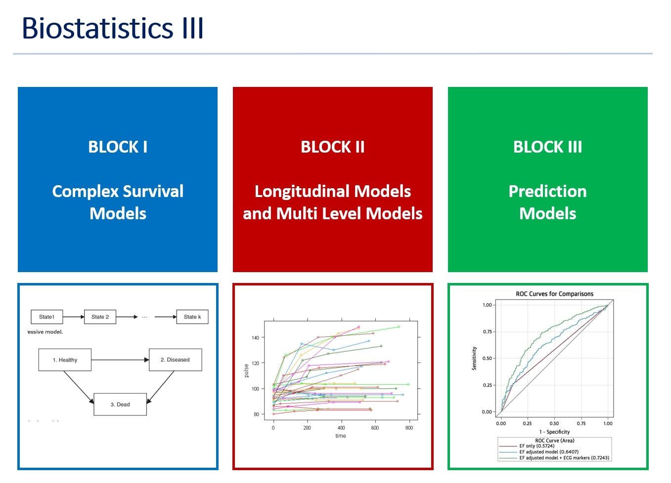
Course overview
1. Core lecture blocks
Advanced topics on Survival Analysis
time-varying coxph model and competing risks
multi-state models
recurrent events
Longitudinal data and multi-level data
linear mixed effect models
GEE
guest lecture on joint modelling of longitudinal data and time-to-event data
Predictive models
clinical predictive modelling for binary outcome
clinical predictive modelling for survival outcome
guest lecture on predictive modelling with machine learning
Additional topics
clinical observational studies
subgroup analysis and heterogeneous treatment effect
2. Motivation of Biostatistics III
Learn advance statistical modelling approaches for observational study and apply to your own research
writing publications that uses these methods, content knowledge to answer reviewer’s questions, as well as reviewing others work/project
building teamwork and collaborative experience
Understanding the importance of statistics in clinical and public health research
which analysis to apply when
how to address data limitations
feasibility and generalization
validity, accuracy, and fit
The aim of the course is to help you
design a complex observational study
develop statistical analysis plan
execute more advanced analyses
interpret outcome and report results
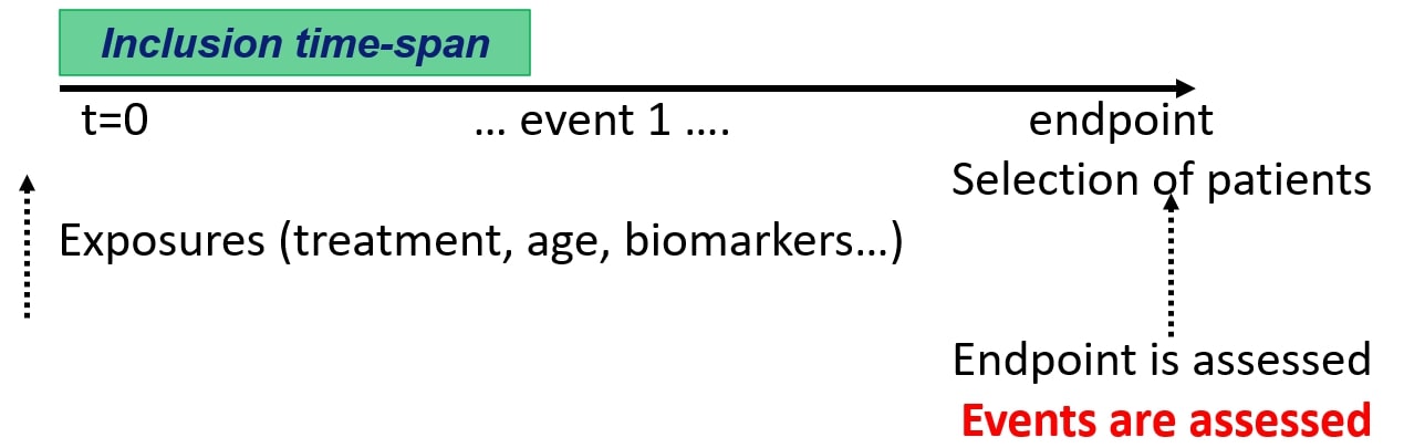
Observational study
1. BASIC points for designing research study (from Victor, Biostat II)
Identify the primary hypothesis: Start simple: if multiple, choose one get it done, and repeat
Determine the form of the primary outcome variable
Identify any potential adjustments that need to made to the analysis
Be honest with yourself
Is there natural or forced clustering of sampled units
Are there important multi-level interactions
Determine primary study variable (predictor/independent variable) and its form
Perform simple analyses
Note that simple does not necessarily mean easy
If clustering needs to be taken into account in the regression, it needs to be taken into account in the basic statistics as well
Determine if you want to use study sample, analytic sample, or both
Perform regressions
Verify that assumptions hold
Where assumptions do not hold, determine if violation is severe enough to warrant adjustment
Last but not least, reporting of observational studies in epidemiology, the STROEB guideline and checklist, https://www.strobe-statement.org/. link to pdf
Survival analysis review
Survival analysis is the study of survival times and of the factors that influence them.
Survival studies can involve
estimation of the survival distribution,
comparisons of the survival distributions of various treatments or interventions,
identification of the factors that influence survival times (inference)
prediction of survival probability and time (prediction)
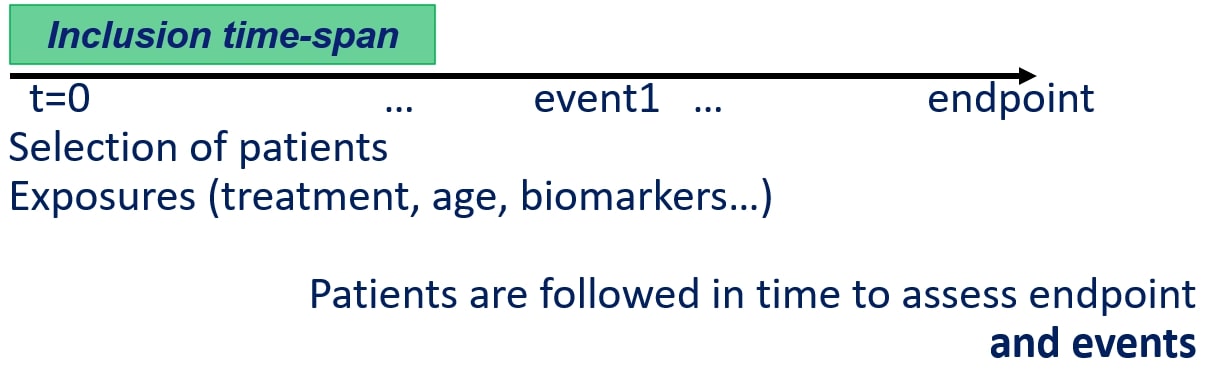
1. Survival data and censoring
Survival Data
response variable is a non-negative discrete or continuous random variable, and represents the time from a well-defined origin to a well-defined event
(time, event), also called time-to-event data
Censoring classification
censoring arises when the starting or ending events are not precisely observed
most common type of censoring is right censoring where final endpoint is only known to exceed a particular value.
less common type of censoring is left censoring where events are known to have occurred before a certain time
interval censoring, where the failure time is only known to have occurred within in a specified interval of time
Type I
censoring times are pre-specified, e.g., a pre-specified ending time
right-censored
Type II
experimental objects are followed until a pre-specified fraction have failed, e.g., until 20% of the study participant experienced the event. less common in medical and public health research
right-censored
Random (or non-informative)
each subject has a censoring time that is statistically independent of their failure time
the observed time value is the minimum of the censoring and failure times
subjects whose failure time is greater than their censoring time are right-censored.
informative censoring can lead to biased survival estimates
patient dropout for non-disease related reasons vs disease related reason
can you assume independence between the event of interest and competing events?
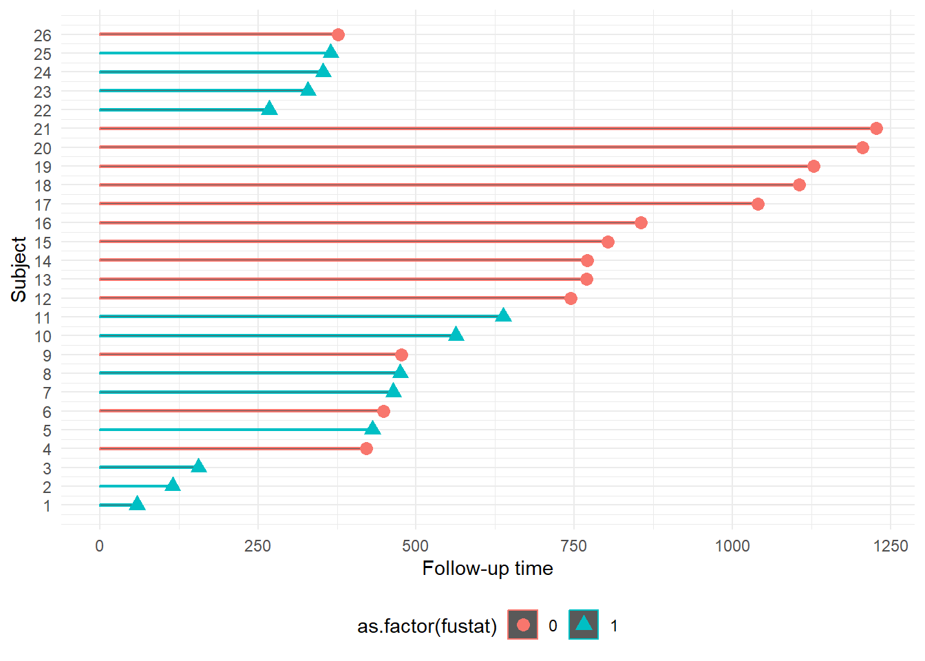
Example survival data, Survival in a randomised trial comparing two treatments for ovarian cancer
Source: Edmunson, J.H., Fleming, T.R., Decker, D.G., Malkasian, G.D., Jefferies, J.A., Webb, M.J., and Kvols, L.K., Different Chemotherapeutic Sensitivities and Host Factors Affecting Prognosis in Advanced Ovarian Carcinoma vs. Minimal Residual Disease. Cancer Treatment Reports, 63:241-47, 1979.
futime: survival or censoring time
fustat: event status (1=event, 0=censoring)
age: in years
resid.ds: residual disease present (1=no,2=yes)
rx: treatment group
ecog.ps: ECOG performance status (1 is better, see reference)
#loading packages;library(survival)library(tidyverse)#display the first 6 rows of data;head(ovarian)
# plot with shapes to indicate censoring or eventovarian2 <- ovarian %>%mutate(Subject =1:length(ovarian$fustat))ggplot(ovarian2, aes(Subject, futime, color =as.factor(fustat))) +geom_bar(stat ="identity", width =0.1) +geom_point(data = ovarian2, aes(Subject, futime, color =as.factor(fustat),shape =as.factor(fustat)), size =3) +scale_x_continuous(breaks =1:length(ovarian$fustat)) +ylab("Follow-up time") +coord_flip() +theme_minimal() +theme(legend.position ="bottom")
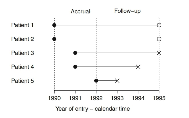
Excercises from Dirk F. Moore, 2016
Consider a simple example of five cancer patients who enter a clinical trial as illustrated in the following diagram:
Create a simple survival data based on this diagram
data to include, patient ID, cohort entry year, survival time and censoring indicator
Identify total number of patients who experienced the event within the study window.
Calculate total person-years and the death rate per person-year
2. Basic Concepts and Principles of Survival Analysis
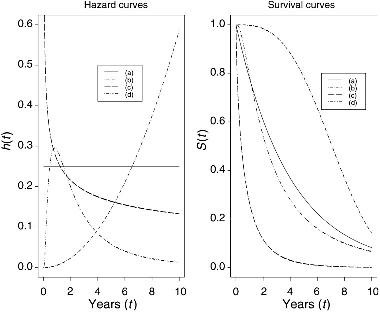
The Hazard and Survival Functions
Survival function: probability of survival beyond time t.
Failure function: probability of event by time t
\[
S(t) = Pr(T>t), 0 < t < \infty
\]
\[
F(t) = 1 - S(t)
\] - Median Survival Time, \(S(t) = 1/2\).
Hazard function: instantaneous failure rate; the probability that, given that a subject has survived up to time t, they fail in the next small interval of time, divide by the length of that interval.
Cumulative hazard function: the integral of the hazard, or the area under the hazard function between times 0 and t; the number of events that would be expected for each individual by time t if the event were a repeatable process
3. Nonparametric Survival Curve Estimation and comparison of Survival Distributions
Kaplan-Meier estimator for survival function
\[
\hat{S}(t) = \prod_{i:t_i \leq t}\Big( 1-\hat{q}_i\Big) = \prod_{i:t_i \leq t}\Big( 1- \frac{d_i}{n_i}\Big)
\] where \(n_i\) is the number of subjects at risk at time \(t_i\), and \(d_i\) is the number of individuals who fail at that time.
Kaplan-Meier estimator has a variance expression known as the Greenwood formula (obtained using delta method), which can be used to construct 95% confidence interval of the estimated survival function.
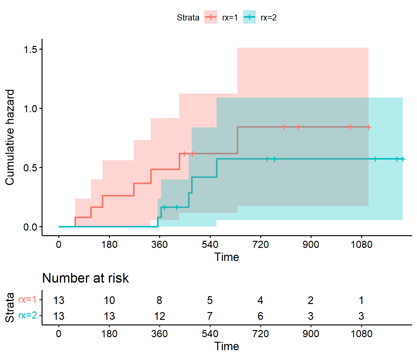
Nelson-Aalen estimator for cumulative hazard function
\[
\hat{H}(t) = \sum_{i:t_i\leq t}\frac{d_i}{n_i}
\] where \(n_i\) is the number of subjects at risk at time \(t_i\), and \(d_i\) is the number of individuals who fail at that time.
less informative than the survival curve
can be used for example for visually checking how constant the hazard rate is over time, since a constant hazard rate corresponds to linear cumulative hazard
Comparing survival functions
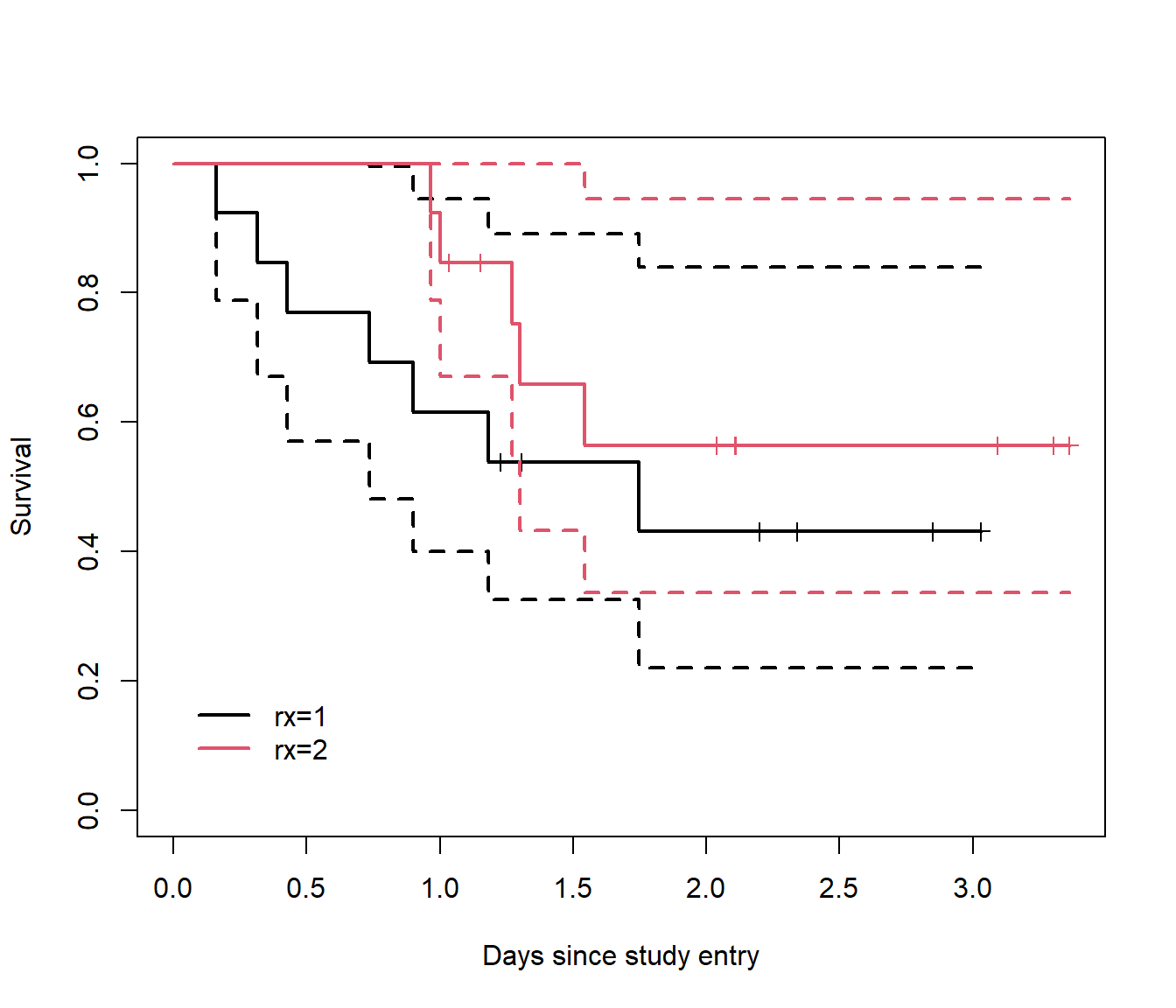
We can plot two or more KM-curves along with their respective confidence bands in the same figure, and see whether the intervals are overlapping at any given point in time.
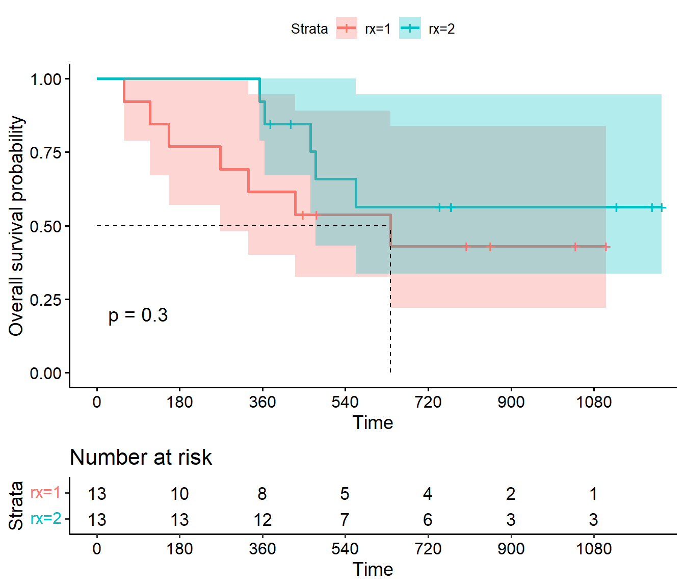
For testing equivalence of two or more survival functions, we can use the non-parametric log-rank test.
log-rank test statistic aggregates the observed and expected event counts in each group and follows a \(\chi^2\) distribution with 1 degree of freedom (2 groups).
We obtain a p-value of 0.3, which is not statistically significant at the 5 % level. There is not enough evidence to conclude difference in survival between the two treatment groups.