log hazard function is expressed in a regression format
\(log(\lambda_0(t))\) can be viewed as intercept
models parameters \(\beta_1, \ldots, \beta_k\) are the log hazard ratios that explain the difference on the hazard of event by varying values of the corresponding covariates
covariates can be continuous, discrete, time-varying, and possible interactions
\(\lambda_0(t)\) is called baseline hazard function
it reflects the underlying hazard for individuals with all covariates set to 0 (“reference group”)
one attractive feature of the Cox model framework is its ability to estimate \(\beta\) without \(\lambda_0(t)\).
\(\lambda_0(t)\) is estimated non-parametrically (i.e., no assumption on its distribution) using Breslow estimator
Cox PH is a semiparametric model.
Assumptions of the Cox Proportional Hazard Model
Independent observations
in the presence of correlated data, one can adjust for cluster correlation using robust variance formula similar to generalized estimating equation (adjustment on the variance of the hazard function), one can also fit frailty terms (random effects) in Cox model - frailty model and estimate these random effects.
Non-informative or independent censoring
independence between the probability of censoring and the event of interest
depending on the types of informative censoring, one can either adjust for the covariates that are believed to cause informative censoring or in some cases consider fitting a competing risks model
Proportional hazard assumption
the ratio of hazard functions (i.e., the relative hazard) is constant over time
we can check for PH assumption violation
when PH assumption is violated, one can consider stratification on the covariates in question or fitting time-varying models.
3. COX PH model in R
library(survival)args(coxph)
function (formula, data, weights, subset, na.action, init, control,
    ties = c("efron", "breslow", "exact"), singular.ok = TRUE,
    robust, model = FALSE, x = FALSE, y = TRUE, tt, method = ties,
    id, cluster, istate, statedata, nocenter = c(-1, 0, 1), ...)
NULL
If robust is TRUE, coxph calculates robust coefficient-variance estimates. The default is FALSE, unless the model includes non-independent observations, specified by the cluster function in the model formula.
NCCTG Lung Cancer Data: Survival in patients with advanced lung cancer from the North Central Cancer Treatment Group. Performance scores rate how well the patient can perform usual daily activities.
inst: Institution code
time: Survival time in days
status: censoring status 1=censored, 2=dead
age: Age in years
sex: Male=1 Female=2
ph.ecog: ECOG performance score as rated by the physician.
0= asymptomatic,
1= symptomatic but completely ambulatory,
2= in bed <50% of the day,
3= in bed > 50% of the day but not bedbound,
4 = bedbound
ph.karno: Karnofsky performance score (bad=0-good=100) rated by physician
pat.karno: Karnofsky performance score as rated by patient
meal.cal: Calories consumed at meals
wt.loss: Weight loss in last six months (pounds)
library(tidyverse)library(gtsummary)#checking data and variable status;str(lung)
'data.frame':   228 obs. of  10 variables:
 $ inst     : num  3 3 3 5 1 12 7 11 1 7 ...
 $ time     : num  306 455 1010 210 883 ...
 $ status   : num  2 2 1 2 2 1 2 2 2 2 ...
 $ age      : num  74 68 56 57 60 74 68 71 53 61 ...
 $ sex      : num  1 1 1 1 1 1 2 2 1 1 ...
 $ ph.ecog  : num  1 0 0 1 0 1 2 2 1 2 ...
 $ ph.karno : num  90 90 90 90 100 50 70 60 70 70 ...
 $ pat.karno: num  100 90 90 60 90 80 60 80 80 70 ...
 $ meal.cal : num  1175 1225 NA 1150 NA ...
 $ wt.loss  : num  NA 15 15 11 0 0 10 1 16 34 ...
#simple way to check for missing column in R;colSums(is.na(lung))
     inst      time    status       age       sex   ph.ecog  ph.karno pat.karno
        1         0         0         0         0         1         1         3
 meal.cal   wt.loss
       47        14
#display summary table on R Markdown files;lung %>%select(-inst) %>%tbl_summary(by = status,missing_text ="(Missing)") %>%add_overall()
Characteristic
Overall
N = 2281
1
N = 631
2
N = 1651
time
256 (167, 399)
284 (221, 444)
226 (135, 387)
age
63 (56, 69)
62 (55, 67)
64 (57, 70)
sex
1
138 (61%)
26 (41%)
112 (68%)
2
90 (39%)
37 (59%)
53 (32%)
ph.ecog
0
63 (28%)
26 (41%)
37 (23%)
1
113 (50%)
31 (49%)
82 (50%)
2
50 (22%)
6 (9.5%)
44 (27%)
3
1 (0.4%)
0 (0%)
1 (0.6%)
(Missing)
1
0
1
ph.karno
50
6 (2.6%)
1 (1.6%)
5 (3.0%)
60
19 (8.4%)
3 (4.8%)
16 (9.8%)
70
32 (14%)
3 (4.8%)
29 (18%)
80
67 (30%)
20 (32%)
47 (29%)
90
74 (33%)
25 (40%)
49 (30%)
100
29 (13%)
11 (17%)
18 (11%)
(Missing)
1
0
1
pat.karno
30
2 (0.9%)
1 (1.6%)
1 (0.6%)
40
2 (0.9%)
1 (1.6%)
1 (0.6%)
50
4 (1.8%)
0 (0%)
4 (2.5%)
60
30 (13%)
3 (4.8%)
27 (17%)
70
41 (18%)
10 (16%)
31 (19%)
80
51 (23%)
12 (19%)
39 (24%)
90
60 (27%)
22 (35%)
38 (23%)
100
35 (16%)
14 (22%)
21 (13%)
(Missing)
3
0
3
meal.cal
975 (635, 1,150)
975 (588, 1,075)
1,025 (675, 1,175)
(Missing)
47
16
31
wt.loss
7 (0, 16)
4 (0, 15)
8 (0, 17)
(Missing)
14
1
13
1 Median (Q1, Q3); n (%)
#removing observation with any missing data;lung2 <- lung %>%filter(complete.cases(.)) %>%mutate(sex =as.factor(sex),ph.ecog =as.factor(ph.ecog))# Model1: full non-interaction additive model;fit1 <-coxph(Surv(time, status) ~ age + sex + ph.ecog + ph.karno + pat.karno + meal.cal + wt.loss , data = lung2)# Model2: excluding predictor pat.karno (nested under Model1);fit2 <-coxph(Surv(time, status) ~ age + sex + ph.ecog + ph.karno + meal.cal + wt.loss, data = lung2)# Model3: full non-interaction additive model with inst as cluster for robust variance estimator;fit3 <-coxph(Surv(time, status) ~ age + sex + ph.ecog + ph.karno + meal.cal + wt.loss +cluster(inst), data = lung2)# Model4: full non-interaction additive model with spline for continuous variable age;fit4 <-coxph(Surv(time, status) ~pspline(age,3) + sex + ph.ecog + ph.karno + meal.cal + wt.loss, data = lung2)fit1
Call:
coxph(formula = Surv(time, status) ~ age + sex + ph.ecog + ph.karno +
    pat.karno + meal.cal + wt.loss, data = lung2)

                coef  exp(coef)   se(coef)      z       p
age        9.979e-03  1.010e+00  1.173e-02  0.851 0.39503
sex2      -5.489e-01  5.776e-01  2.023e-01 -2.713 0.00667
ph.ecog1   6.470e-01  1.910e+00  2.822e-01  2.293 0.02187
ph.ecog2   1.454e+00  4.282e+00  4.621e-01  3.147 0.00165
ph.ecog3   2.762e+00  1.584e+01  1.123e+00  2.460 0.01389
ph.karno   2.207e-02  1.022e+00  1.132e-02  1.949 0.05128
pat.karno -1.150e-02  9.886e-01  8.579e-03 -1.340 0.18013
meal.cal   2.752e-05  1.000e+00  2.609e-04  0.105 0.91601
wt.loss   -1.436e-02  9.857e-01  7.835e-03 -1.833 0.06681

Likelihood ratio test=28.63  on 9 df, p=0.000748
n= 167, number of events= 120
# display regression output in R markdown;fit1 %>%tbl_regression(exp=TRUE)
Characteristic
HR
95% CI
p-value
age
1.01
0.99, 1.03
0.4
sex
1
—
—
2
0.58
0.39, 0.86
0.007
ph.ecog
0
—
—
1
1.91
1.10, 3.32
0.022
2
4.28
1.73, 10.6
0.002
3
15.8
1.75, 143
0.014
ph.karno
1.02
1.00, 1.05
0.051
pat.karno
0.99
0.97, 1.01
0.2
meal.cal
1.00
1.00, 1.00
>0.9
wt.loss
0.99
0.97, 1.00
0.067
Abbreviations: CI = Confidence Interval, HR = Hazard Ratio
# checking goodness-of-fit;# Akaike Information Criterion;AIC(fit1)
[1] 1005.604
AIC(fit2) #the smaller the better;
[1] 1005.379
AIC(fit3) #likelihood don't change under robust variance;
[1] 1005.379
AIC(fit4) #it seems age non-linear fits slightly better;
[1] 1005.127
# comparing between nested models;# using likelihood ratio test;anova(fit1, fit2)
Analysis of Deviance Table
 Cox model: response is  Surv(time, status)
 Model 1: ~ age + sex + ph.ecog + ph.karno + pat.karno + meal.cal + wt.loss
 Model 2: ~ age + sex + ph.ecog + ph.karno + meal.cal + wt.loss
   loglik  Chisq Df Pr(>|Chi|)
1 -493.80
2 -494.69 1.7759  1     0.1827
anova(fit1, fit4)
Analysis of Deviance Table
 Cox model: response is  Surv(time, status)
 Model 1: ~ age + sex + ph.ecog + ph.karno + pat.karno + meal.cal + wt.loss
 Model 2: ~ pspline(age, 3) + sex + ph.ecog + ph.karno + meal.cal + wt.loss
   loglik  Chisq     Df Pr(>|Chi|)
1 -493.80
2 -492.54 2.5303 1.0268     0.1157
anova(fit2, fit4)
Analysis of Deviance Table
 Cox model: response is  Surv(time, status)
 Model 1: ~ age + sex + ph.ecog + ph.karno + meal.cal + wt.loss
 Model 2: ~ pspline(age, 3) + sex + ph.ecog + ph.karno + meal.cal + wt.loss
   loglik  Chisq     Df Pr(>|Chi|)
1 -494.69
2 -492.54 4.3062 2.0268     0.1188
#LRT test revealed that model without pat.karno and spline does not change the fit significantly, we can keep the simpler model;# checking c-statistics;#you can compute Wald confidence interval of C-index;# pointest +/- 1.96*se; For example, for model 1, we havepaste(0.654-1.96*0.029, 0.654+1.96*0.029, sep =",")
[1] "0.59716,0.71084"
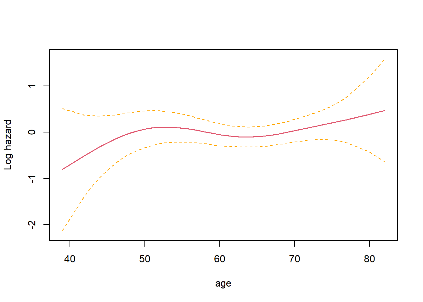
# we can visulize the spline fit for variable age;# terms=, specify the index order of the variable we wish to plot;termplot(fit4, se=T, terms=1, ylabs="Log hazard")
we cannot use anova() to conduct likelihood ratio test with clustered data, however, adding a cluster term using cluster() does not change the loglikelihood of the model (hence the observed identical value of AIC between fit2 and fit3)
Note that, \(k\) represents number of parameters in the model and \(l(\cdot)\) is the partial loglikelihood of a specified model.
\[
AIC = -2 \times l(\hat{\beta}) + 2 \times k
\]
Cox PH model diangostics
Model diagnostic residuals
(linearity): Martingale residuals and Deviance residuals
(influential observations): Score residuals and dfbeta measures
(proportional hazard): Schoenfeld residuals
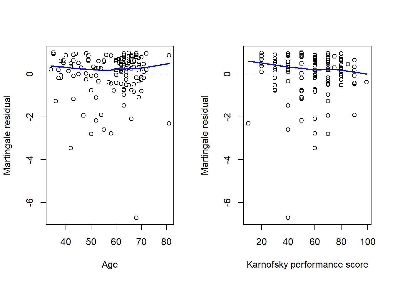
1. Martingale residuals and Deviance residuals (linearity)
\[
M_i(t) = N_i(t) - \int_0^t Y_i(u)exp\{\beta'x_i\} \lambda_0 (u)du
\] - can be view as the difference between the observed event process and the model estimated event process
The \(\hat{M}_i\) for \(i=1, \ldots, n\) can be plotted against continuous covariates to check for non-linearity of the covariate effects.
This is because any systematic deviation from linearity (on the modelled log hazard ratio) will show as systematic difference in the residuals.
If there is evidence of linearity violation - that is an additive linear combination of the covariates a not suitable, we can consider including interactions, higher order terms, splines and other function forms etc.
Deviance residuals are re-scaled versions of martingale residuals, to make them more symmetric around zero.
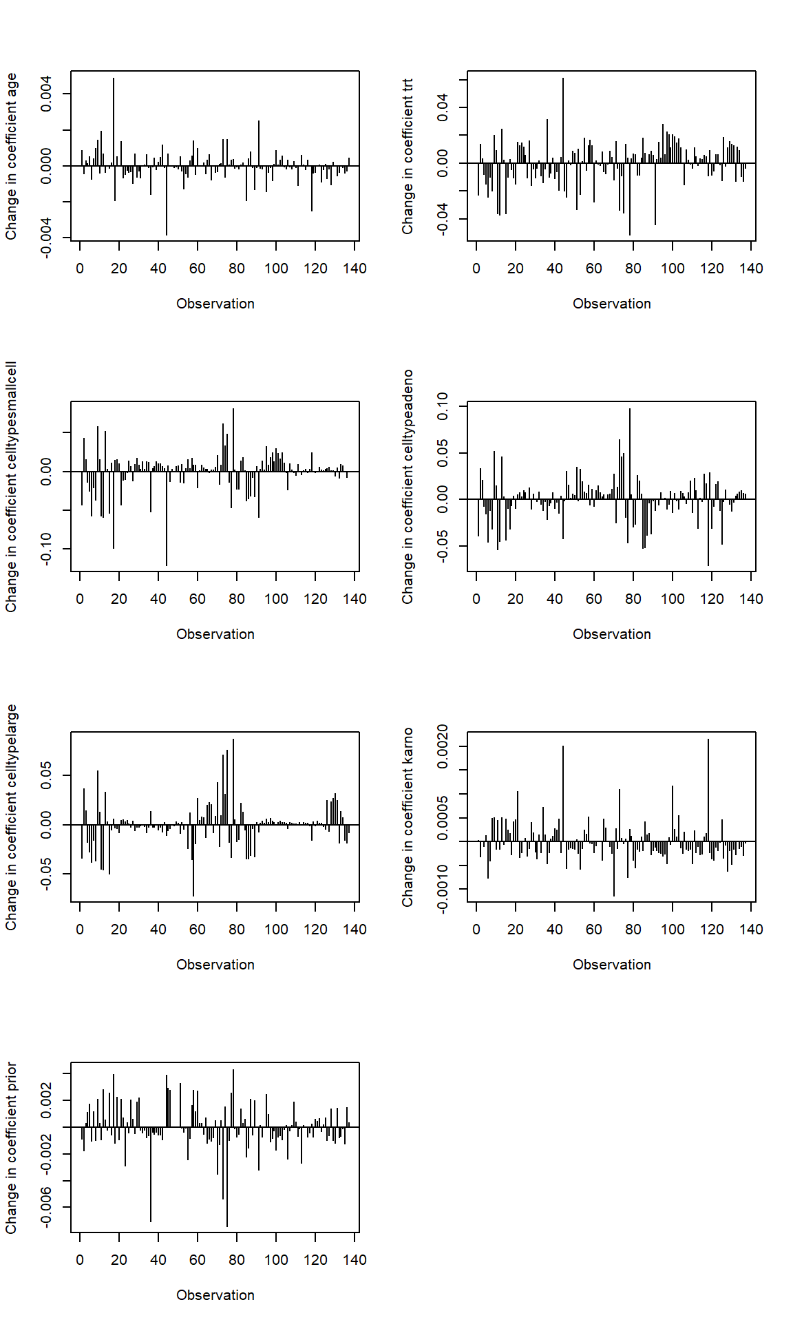
2. Score residual and dfbeta measure (influential observations)
Some subjects may have an especially large influence on the parameter estimates. It is helpful for the data analyst to have tools that can identify those subjects.
Score residual and dfbeta measure the influence of the observation \(i\) on the parameter estimates when \(i\) is removed from the model fit. These are calculated separately for each regression coefficient.
We can conduct sensitivity analysis by comparing the estimated log Hazard ratios (the Cox regression coefficients) with and without the identified influential observations.
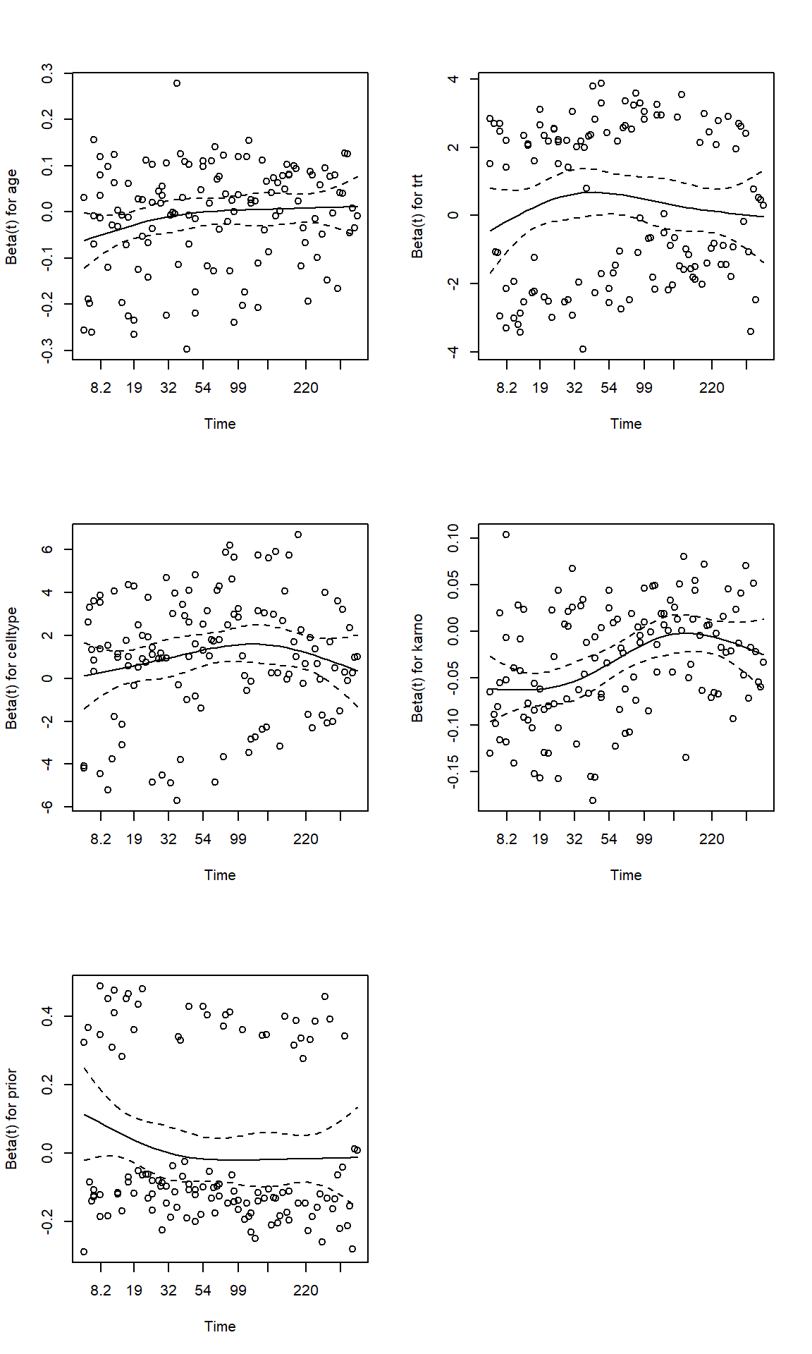
3. Schoenfeld residuals (proportional hazard)
Schoenfeld residuals are defined from the score function as \[
\hat{r}_i(t) = x_i(t) - \frac{\sum_{l=1}^n Y_l(t)exp(\hat{\beta}'x_l(t)) x_l(t) }{\sum_{l=1}^n Y_l(t)exp(\hat{\beta}'x_l(t)) },
\]
can be seen as the difference between the observed covariate and the expected covariate at each failure time.
the expected covariate is a weighted-average of the covariate, weighted by each individual’s likelihood of event at \(t\).
Schoenfeld residuals are calculated for each covariates and are defined only for non-censored observations
Schoenfeld (1982) showed that these residuals are asymptotically uncorrelated and have expectation valued at 0. Thus a plot of Schoenfeld residuals against time should be centered around zero.
In principle, a Schoenfeld residuals plot that shows a non-random pattern against time is evidence of violation of the PH assumption.
4. More on proportional hazard assumptions
In addition to plotting the Schoenfeld residuals against time, we can also use the cox.zph() function to check for PH assumption of a fitted Cox model.
Another way to test PH would be to add covariate-time interaction terms into the model, and test whether these are significantly different from 0.
Randomised trial of two treatment regimens for lung cancer. This is a standard survival analysis data set.
D Kalbfleisch and RL Prentice (1980), The Statistical Analysis of Failure Time Data. Wiley, New York.
# calculating residuals from fox model;fit <-coxph(Surv(time, status) ~ age + trt + celltype + karno + prior, data = veteran)fit %>%tbl_regression(exp=FALSE)
Characteristic
log(HR)
95% CI
p-value
age
-0.01
-0.03, 0.01
0.3
trt
0.29
-0.11, 0.70
0.2
celltype
squamous
—
—
smallcell
0.86
0.33, 1.4
0.002
adeno
1.2
0.61, 1.8
<0.001
large
0.40
-0.15, 0.96
0.2
karno
-0.03
-0.04, -0.02
<0.001
prior
0.01
-0.03, 0.05
0.7
Abbreviations: CI = Confidence Interval, HR = Hazard Ratio
# dfbetaindex.obs <-1:length(veteran$time)par(mfrow=c(4,2))for (i in1:length(fit$coefficients)){plot(dfbeta[,i] ~ index.obs, type="h",xlab="Observation", ylab=paste("Change in coefficient", names(fit$coefficients)[i], sep =" "))abline(h=0)}#return observations are influential#where the log(HR) on age changes more than 15% of the model estimated value at 0.01;which(abs(dfbeta[,1])>0.01*0.15)
fit2<-coxph(Surv(tstart, time, status) ~ age + trt*strata(celltype) + karno:strata(tgroup) + prior, data=vet2)fit2
Call:
coxph(formula = Surv(tstart, time, status) ~ age + trt * strata(celltype) +
    karno:strata(tgroup) + prior, data = vet2)

                                   coef exp(coef)  se(coef)      z        p
age                           -0.012305  0.987770  0.009765 -1.260   0.2076
trt                           -0.404353  0.667409  0.414695 -0.975   0.3295
prior                          0.006850  1.006874  0.021471  0.319   0.7497
trt:strata(celltype)smallcell  0.897756  2.454089  0.534178  1.681   0.0928
trt:strata(celltype)adeno      0.242645  1.274616  0.621954  0.390   0.6964
trt:strata(celltype)large      0.848816  2.336879  0.589146  1.441   0.1497
karno:strata(tgroup)tgroup=1  -0.048355  0.952796  0.006758 -7.155 8.35e-13
karno:strata(tgroup)tgroup=2   0.011038  1.011100  0.015801  0.699   0.4848
karno:strata(tgroup)tgroup=3  -0.016906  0.983236  0.020528 -0.824   0.4102

Likelihood ratio test=60.89  on 9 df, p=9.03e-10
n= 225, number of events= 128
cox.zph(fit2)
                      chisq df     p
age                   4.122  1 0.042
trt                   0.186  1 0.667
prior                 2.260  1 0.133
trt:strata(celltype)  3.774  3 0.287
karno:strata(tgroup)  2.207  3 0.531
GLOBAL               14.382  9 0.109
Time Dependent Covariates
1. Immortal Time Bias
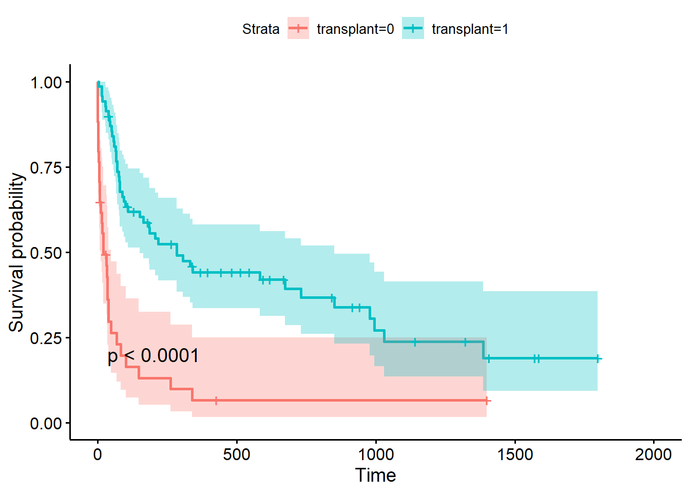
We might be interested to know if the ones who received transplant have better survival outcome than those who don’t.
We can check the Kaplan Meier curve of Survival between the transplant receivers and the non receivers.
The plot shows that receivers have clear better survival than those who received transplant.
library(survminer)fit<-survfit(Surv(futime, fustat) ~ transplant, data = jasa)ggsurvplot(fit = fit, data = jasa, conf.int =TRUE, pval =TRUE)
This result may appear to indicate (as it did to Clark et al. in 1971) that transplants are extremely effective in increasing survival of the recipients.
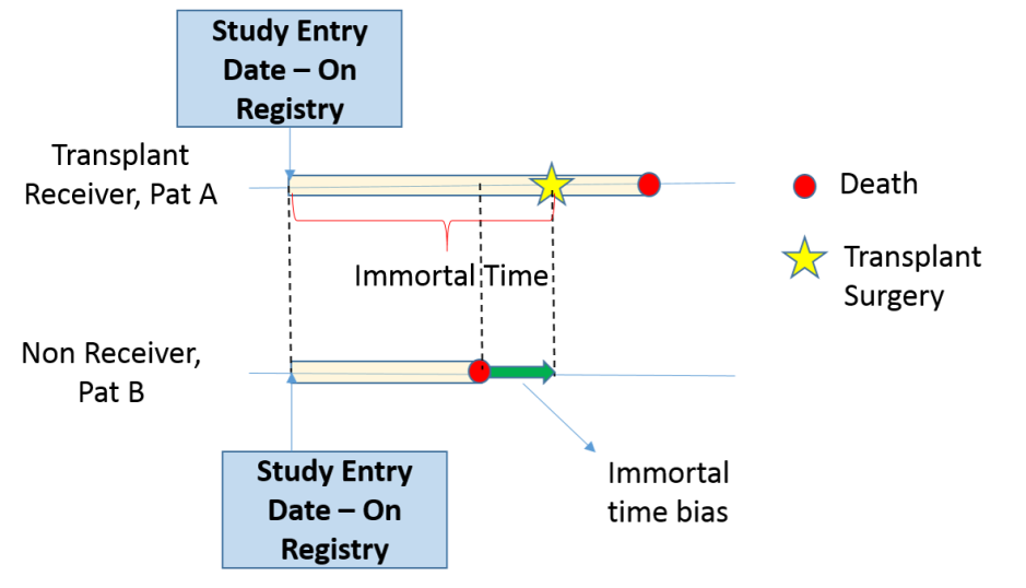
The problem here is that receipt of a transplant is a time dependent covariate;
patients who received a transplant had to live long enough to receive that transplant. (immortal time bias)
“landmark” analysis, analyze the effect prior to receiving transplant and after receiving transplant.
Home reading - the oscar study
Oscar winning actors and actresses live longer than their less successful peers.
If we study the survival of winners versus nominees, we are looking at survival conditioning on something happened in the future.
Those winners are guaranteed to survive until their winning, resulting a immortal time window.
2. Handle time-dependent covariates in Cox PH model
1. The Stanford Heart Transplant data
Survival of patients on the waiting list for the Stanford heart transplant program.
J Crowley and M Hu (1977), Covariance analysis of heart transplant survival data. Journal of the American Statistical Association, 72, 27-36.
To proceed with time-dependent analysis, we want to create transplant as a time-dependent covariates.
we need to create a new dataset that add a new data line representing the time when a transplant occurred - wide to long data.
we can use the tmerge() function in the survival package to create multiple time-based intervals per subject
# step 1: adding subject identifier to the data;jasa <- jasa %>%mutate(id =1:nrow(jasa),age =round(age,2))# step 2: check if there is any event time that is 0;# we need to update this to 0.5, representing event happened mid-day;# the analysis cannot handle an event time at the start of the study;which(jasa$futime==0)
[1] 15
jasa[which(jasa$futime==0), "futime"] <-0.5# Step 3: create multiple entries for each subject by transplant status and time;jasa_new <-tmerge(data1 = jasa[,c("id", "age","accept.dt","surgery")], #data1 is the baseline data to be retained in the analysis (time-independent);data2 = jasa[,c("id","transplant","wait.time","futime","fustat")],#data2 is source for new data including events and time-dependent var;id = id, #subject identifier used to merge the data together;death =event(futime, fustat),transplant=tdc(wait.time))datatable(jasa_new,rownames =FALSE,options =list(dom ='t'))
New we can fit a time-dependent COX model
we are interested in investigating the effect of transplant on survival
we would like to also adjust for age at study entry, year of study entry prior or post 1970 (cohort effect), prior bypass surgery status
#creating a new variable called year for cohort entry year;jasa_new$year =ifelse(format(as.Date(jasa_new$accept.dt, format="%d/%m/%Y"),"%Y")<1970,0,1)# correct time-dependent analysis;fit_correct <-coxph(Surv(tstart, tstop, death) ~ age + transplant + surgery, data = jasa_new)fit_correct
Call:
coxph(formula = Surv(tstart, tstop, death) ~ age + transplant +
    surgery, data = jasa_new)

               coef exp(coef) se(coef)      z      p
age         0.03139   1.03188  0.01392  2.254 0.0242
transplant -0.07898   0.92406  0.30608 -0.258 0.7964
surgery    -0.77035   0.46285  0.35959 -2.142 0.0322

Likelihood ratio test=10.78  on 3 df, p=0.01295
n= 169, number of events= 75
# incorrect analysis using the original data;fit_incorrect <-coxph(Surv(futime, fustat) ~ age + transplant + surgery, data = jasa)fit_incorrect
Call:
coxph(formula = Surv(futime, fustat) ~ age + transplant + surgery,
    data = jasa)

               coef exp(coef) se(coef)      z        p
age         0.05890   1.06067  0.01505  3.914 9.10e-05
transplant -1.71722   0.17956  0.27854 -6.165 7.04e-10
surgery    -0.41899   0.65771  0.37118 -1.129    0.259

Likelihood ratio test=45.85  on 3 df, p=6.089e-10
n= 103, number of events= 75
The correct analysis shows that transplant is not statistically significant at improving survival!
2. Mayo Clinic Primary Biliary Cirrhosis, sequential data
This data is a continuation of the PBC data set, and contains the follow-up laboratory data for each study patient. An analysis based on the data can be found in Murtagh, et. al. (1994)
Murtaugh PA. Dickson ER. Van Dam GM. Malinchoc M. Grambsch PM. Langworthy AL. Gips CH. “Primary biliary cirrhosis: prediction of short-term survival based on repeated patient visits.” Hepatology. 20(1.1):126-34, 1994.
id: case number
age: in years
sex: m/f
trt: 1/2/NA for D-penicillmain, placebo, not randomised
time: number of days between registration and the earlier of death,
transplantion, or study analysis in July, 1986
status: status at endpoint, 0/1/2 for censored, transplant, dead
day: number of days between enrollment and this visit date
all measurements below refer to this date
albumin: serum albumin (mg/dl)
alk.phos: alkaline phosphotase (U/liter)
ascites: presence of ascites
ast: aspartate aminotransferase, once called SGOT (U/ml)
bili: serum bilirunbin (mg/dl)
chol: serum cholesterol (mg/dl)
copper: urine copper (ug/day)
edema: 0 no edema, 0.5 untreated or successfully treated 1 edema despite diuretic therapy
hepato: presence of hepatomegaly or enlarged liver
There are three event status, we can treat the data as a multi-state problem (if we are interested in estimating the hazard rate between each status change).
In the original paper, the primary analysis focus on death, patients were censored at the time of transplantation!
The analysis below is to demonstrate how you would fit Cox model with follow-up repeatedly measured lab values where we censore patient if they received transplant;
pbcseq2 <- pbcseq %>%group_by(id) %>%mutate(tstart = day, tstop =lead(day)) # impute the last missing lead value with the end of follow up time;pbcseq2$tstop[is.na(pbcseq2$tstop)] <- pbcseq2$futime[is.na(pbcseq2$tstop)]fit_example <-coxph(Surv(tstart, tstop, status==2) ~ age + sex + trt + albumin + bili, data = pbcseq2)fit_example %>%tbl_regression(exp=TRUE)
Characteristic
HR
95% CI
p-value
age
1.03
1.02, 1.04
<0.001
sex
m
—
—
f
0.56
0.46, 0.68
<0.001
trt
0.92
0.80, 1.07
0.3
albumin
0.45
0.39, 0.53
<0.001
bili
1.09
1.08, 1.10
<0.001
Abbreviations: CI = Confidence Interval, HR = Hazard Ratio
Summary
Cox model aims to estimate risk score of the event to each subject that best predicts the outcome based on
risk set: which subjects experienced what event and which subjects are still at risk of experience an event
covariates values of each subject just prior to the event time.
we use these info to construct time-based data to reflect changes in covariates over study period, and fit time-dependent Cox model.