Predictive modelling lab2

1. Hands-on excerise building a predictive model for time-to-event data using COX PH model

1.1 Descriptive analysis

• For this tutorial, we will be using the HBV data. This data set contains information on the follow-up of untreated hepatitis B patients (natural disease course) with advanced fibrosis/cirrhosis.

• The time-to-event outcome is defined using HCC and HCC_T,

• Predictors considered are: AGE, SEX, HBEAG, SPLENO, BILIRUB, AST, ALT, PLAT, ALBUMIN, GAMMA

• The data are as follows:

  • SUBJECTID: ID code
  • HBEAG: HBeAg positive =1 or negative=0
  • AGE: age at diagnose (year)
  • SEX: 0 = female; 1 = male
  • SPLENO: splenomegany 0=no 1=yes
  • BILIRUB: bilirubin
  • AST
  • ALT
  • PLAT: platelet count
  • ALBUMIN: albumin
  • GAMMA: GGT
  • HCC: development of hepatocellular carcinoma 0=no 1 =yes
  • HCC_T: time to HCC (months)

library(tidyverse)
library(gtsummary)
library(DT)
options(scipen = 999)

hbv <- read.csv("HBV.csv", header = TRUE,fileEncoding="UTF-8-BOM")

# look at new data;
datatable(hbv,
          rownames = FALSE,
          options = list(dom = 't')) 

# display summary statistics by survival status;
hbv[,-1] %>% 
  tbl_summary(
  by = HCC,
  missing_text = "(Missing)") %>%
  add_overall() %>%
  add_p()

Characteristic	Overall N = 161 1	0 N = 108 1	1 N = 53 1	p-value 2
HBEAG	45 (28%)	31 (29%)	14 (26%)	0.8
AGE	47 (38, 56)	46 (37, 54)	53 (40, 60)	0.005
SEX	129 (80%)	89 (82%)	40 (75%)	0.3
SPLENO	46 (29%)	23 (21%)	23 (43%)	0.004
BILIRUB	14 (10, 20)	14 (10, 19)	15 (10, 27)	0.10
(Missing)	1	0	1
AST	1.87 (1.00, 3.29)	1.78 (1.00, 2.97)	2.18 (1.43, 3.75)	0.12
ALT	2.6 (1.2, 4.8)	2.6 (1.5, 5.2)	2.6 (1.0, 4.2)	0.4
PLAT	146 (91, 195)	158 (130, 203)	95 (56, 140)	<0.001
(Missing)	1	1	0
ALBUMIN	40 (36, 43)	41 (38, 44)	36 (32, 41)	<0.001
(Missing)	3	3	0
GAMMA	17 (14, 22)	15 (13, 21)	19 (16, 25)	<0.001
HCC_t	72 (32, 98)	82 (53, 106)	40 (19, 72)	<0.001
1 n (%); Median (Q1, Q3)
2 Pearson’s Chi-squared test; Wilcoxon rank sum test

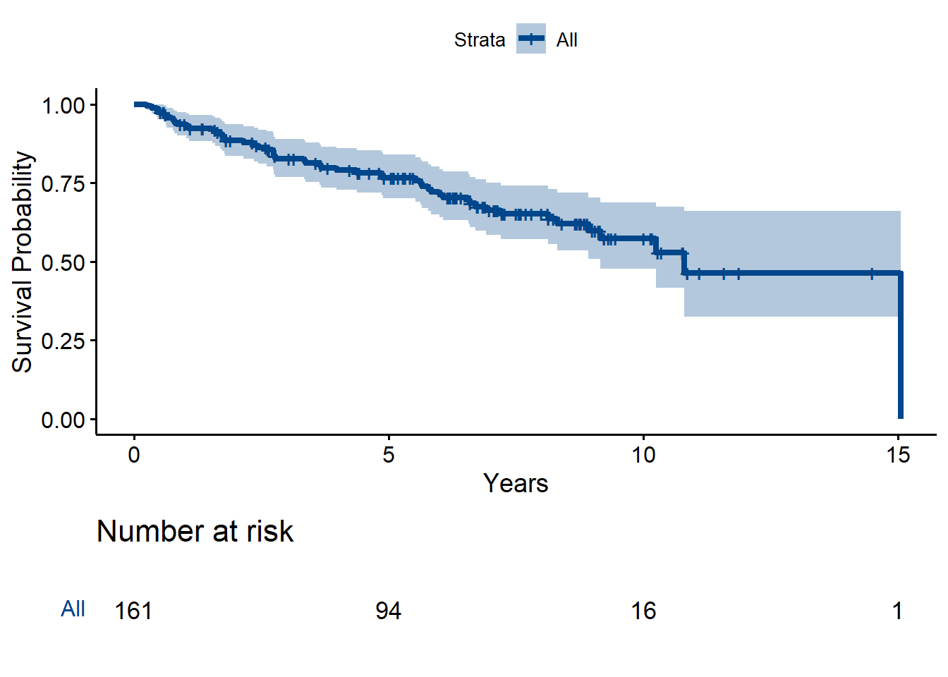
# checking out KM curve;
library(survival)
library(survminer)

m0 <- survfit(Surv(HCC_t/12, HCC) ~ 1, data = hbv) 
m0

Call: survfit(formula = Surv(HCC_t/12, HCC) ~ 1, data = hbv)

       n events median 0.95LCL 0.95UCL
[1,] 161     53   10.8    9.16      NA

ggsurvplot(m0, 
           data = hbv,
           risk.table = TRUE,
           size = 1.5,
           palette = "lancet",
           xlab = "Years",
           ylab = "Survival Probability",
           tables.theme = theme_cleantable())

1.2 Data manipulation

• Although there are missing data, we will proceed with complete analysis.

# complete data;
hbv2 <- hbv[complete.cases(hbv), ]

dim(hbv)

[1] 161  13

dim(hbv2)

[1] 156  13

• Following the Toronto HCC risk index paper Sharma et al (2017), we will categorize the continuous predictors.

# grouping age and platelets;
hbv2 <- hbv2 %>%
  mutate(
    agec = case_when(
      AGE < 45 ~ "<45",
      AGE >=45 & AGE <60 ~ "45-60",
      AGE >= 60 ~ ">60"),
    platc = case_when(
      PLAT < 80 ~"<80",
      PLAT >= 80 & PLAT < 140 ~ "80-139",
      PLAT >= 140 & PLAT < 200 ~ "140-200",
      PLAT >= 200 ~ ">200"
    )) %>%
  mutate(
    HBEAG = as.factor(HBEAG),
    SEX = as.factor(SEX),
    SPLENO = as.factor(SPLENO),
    agec = as.factor(agec),
    platc = as.factor(platc)
  )

1.3 Model building strategies

• Checking the association between predictors and time to hcc via univariate COX PH model

# loop through univariate analysis across a list of predictors;
# checking variable names;
colnames(hbv2)

 [1] "SubjectID" "HBEAG"     "AGE"       "SEX"       "SPLENO"    "BILIRUB"  
 [7] "AST"       "ALT"       "PLAT"      "ALBUMIN"   "GAMMA"     "HCC"      
[13] "HCC_t"     "agec"      "platc"    

predictors <- colnames(hbv2)[c(2:11, 14:15)]
  
#making formulas
univ_formulas <- sapply(predictors,function(x)as.formula(paste('Surv(HCC_t,HCC)~',x)))

#making a list of models;
univ_models <- lapply(univ_formulas,function(x){coxph(x,data=hbv2)})

#extract summary statistics;
univ_results <- lapply(univ_models,function(x){return(summary(x)$coef)})

univ_results

$HBEAG
            coef exp(coef) se(coef)         z  Pr(>|z|)
HBEAG1 0.1705865     1.186 0.314477 0.5424452 0.5875119

$AGE
          coef exp(coef)   se(coef)        z    Pr(>|z|)
AGE 0.03896278  1.039732 0.01230335 3.166843 0.001541036

$SEX
           coef exp(coef)  se(coef)         z   Pr(>|z|)
SEX1 -0.5551918 0.5739622 0.3262331 -1.701826 0.08878808

$SPLENO
             coef exp(coef)  se(coef)        z    Pr(>|z|)
SPLENO1 0.8366366  2.308589 0.2848545 2.937066 0.003313336

$BILIRUB
              coef exp(coef)   se(coef)        z   Pr(>|z|)
BILIRUB 0.02577862  1.026114 0.01227849 2.099494 0.03577342

$AST
          coef exp(coef)   se(coef)         z  Pr(>|z|)
AST 0.02537107  1.025696 0.03969264 0.6391883 0.5227005

$ALT
           coef exp(coef)   se(coef)          z  Pr(>|z|)
ALT -0.02068939 0.9795232 0.03401123 -0.6083105 0.5429815

$PLAT
            coef exp(coef)    se(coef)         z       Pr(>|z|)
PLAT -0.01159488 0.9884721 0.002589088 -4.478365 0.000007521694

$ALBUMIN
               coef exp(coef)   se(coef)         z      Pr(>|z|)
ALBUMIN -0.09143626 0.9126195 0.02120756 -4.311493 0.00001621555

$GAMMA
            coef exp(coef)   se(coef)        z   Pr(>|z|)
GAMMA 0.03095992  1.031444 0.01489857 2.078046 0.03770511

$agec
               coef exp(coef)  se(coef)         z     Pr(>|z|)
agec>60   1.2961524  3.655206 0.3605765 3.5946671 0.0003248066
agec45-60 0.1383743  1.148405 0.3299027 0.4194397 0.6748947962

$platc
                   coef exp(coef)  se(coef)         z     Pr(>|z|)
platc>200    -1.9252340 0.1458416 0.4962241 -3.879767 0.0001045566
platc140-200 -1.3615784 0.2562560 0.3960810 -3.437626 0.0005868373
platc80-139  -0.7942238 0.4519319 0.3357408 -2.365586 0.0180015579

based on the univariate analysis the following predictors are statistically significant: age (and agec), spleno, bilirub, plat (and platc), albumin, gamma.

• perform variable selection using LASSO

library(glmnet)
y <- Surv(hbv2$HCC_t,hbv2$HCC)
x <- model.matrix( ~ AGE + SEX + HBEAG + SPLENO + BILIRUB + AST + ALT + PLAT + ALBUMIN + GAMMA, hbv2)
set.seed(123)
cv.fit <- cv.glmnet(x, y, family="cox", alpha = 1, type.measure = "C") #type.measure="C" is Harrel's concordance measure;

#by cross-validation, we find optimal lambda value that minimizes MSE;
best_lambda <- cv.fit$lambda.min

#we can also use the largest lambda within one standard error of the minimum, leading to a more parsimonious model;
best_lambda2 <- cv.fit$lambda.1se

best_lambda #lambda value that minimizes MSE;

[1] 0.005987403

best_lambda2 #lambda value within 1 standard error of the minimum;

[1] 0.06128292

# extract coefficients of from the best model using min lambda;
coef(cv.fit, s = "lambda.min")

11 x 1 sparse Matrix of class "dgCMatrix"
                       1
(Intercept)  .          
AGE          0.027952059
SEX1        -0.006688095
HBEAG1       0.475707548
SPLENO1      0.294741080
BILIRUB      0.011933437
AST          .          
ALT         -0.028187790
PLAT        -0.007172029
ALBUMIN     -0.081434515
GAMMA        0.020888938

#Visualize coefficients across lambda;
#plot of MSE by lambda;
plot(cv.fit, xvar = "lambda", label = TRUE )
abline(v = log(best_lambda), col = "red", lty = 2)
abline(v = log(best_lambda2), col = "blue", lty = 2)

predictor selection kept the following variables: age, sex, HBEAG, SPLENO, BILIRUB, ALT, PLAT, ALBUMIN, GAMMA

• Fitting our first candidate COX PH model

# selected by LASSO;
hbv2$HCC_ty <- hbv2$HCC_t/12
m1 <- coxph(Surv(HCC_ty, HCC) ~ AGE+factor(SEX)+factor(HBEAG)+factor(SPLENO)+BILIRUB+ALT+PLAT+ALBUMIN+GAMMA, data=hbv2, x=T, y=T)
summary(m1)

Call:
coxph(formula = Surv(HCC_ty, HCC) ~ AGE + factor(SEX) + factor(HBEAG) + 
    factor(SPLENO) + BILIRUB + ALT + PLAT + ALBUMIN + GAMMA, 
    data = hbv2, x = T, y = T)

  n= 156, number of events= 52 

                     coef exp(coef)  se(coef)      z Pr(>|z|)    
AGE              0.029296  1.029730  0.013353  2.194 0.028241 *  
factor(SEX)1    -0.004553  0.995457  0.364121 -0.013 0.990023    
factor(HBEAG)1   0.537761  1.712169  0.338672  1.588 0.112320    
factor(SPLENO)1  0.307000  1.359341  0.313719  0.979 0.327787    
BILIRUB          0.013626  1.013719  0.014215  0.959 0.337793    
ALT             -0.033472  0.967082  0.030894 -1.083 0.278600    
PLAT            -0.007354  0.992673  0.002677 -2.748 0.006005 ** 
ALBUMIN         -0.084967  0.918543  0.025724 -3.303 0.000957 ***
GAMMA            0.023531  1.023810  0.021032  1.119 0.263217    
---
Signif. codes:  0 '***' 0.001 '**' 0.01 '*' 0.05 '.' 0.1 ' ' 1

                exp(coef) exp(-coef) lower .95 upper .95
AGE                1.0297     0.9711    1.0031    1.0570
factor(SEX)1       0.9955     1.0046    0.4876    2.0322
factor(HBEAG)1     1.7122     0.5841    0.8816    3.3253
factor(SPLENO)1    1.3593     0.7357    0.7350    2.5140
BILIRUB            1.0137     0.9865    0.9859    1.0424
ALT                0.9671     1.0340    0.9103    1.0274
PLAT               0.9927     1.0074    0.9875    0.9979
ALBUMIN            0.9185     1.0887    0.8734    0.9660
GAMMA              1.0238     0.9767    0.9825    1.0669

Concordance= 0.766  (se = 0.033 )
Likelihood ratio test= 47.07  on 9 df,   p=0.0000004
Wald test            = 42.87  on 9 df,   p=0.000002
Score (logrank) test = 48.22  on 9 df,   p=0.0000002

• note here the concordance index (C-statistics) is 0.766 with 95% CI (0.70132, 0.83068).

• Check for model fit and model assumptions

# PH assumption;
cox.zph(m1)

                chisq df    p
AGE            0.1365  1 0.71
factor(SEX)    0.6954  1 0.40
factor(HBEAG)  0.0904  1 0.76
factor(SPLENO) 1.5746  1 0.21
BILIRUB        0.8890  1 0.35
ALT            1.1677  1 0.28
PLAT           0.4906  1 0.48
ALBUMIN        1.0105  1 0.31
GAMMA          0.0863  1 0.77
GLOBAL         6.9295  9 0.64

ggcoxdiagnostics(m1, type = "schoenfeld", title = "Diagnostic Plot- PH")

# Linearity;
martingaleresi_plot <- function(x,data=hbv2){
  
data$resid_mart <- residuals(m1, type = "martingale")

ggplot(data = data, aes(x = .data[[x]], y = resid_mart)) +
    geom_point() +
    geom_smooth() +
    theme_bw() + theme(legend.key = element_blank())
  
}

p1<-martingaleresi_plot("AGE")
p2<-martingaleresi_plot("BILIRUB")
p3<-martingaleresi_plot("ALT")
p4<-martingaleresi_plot("PLAT")
p5<-martingaleresi_plot("ALBUMIN")
p6<-martingaleresi_plot("GAMMA")
ggarrange(p1,p2,p3,p4,p5,p6,
          ncol = 3, nrow = 2)

• We could consider log all the lab values.

m2 <- coxph(Surv(HCC_ty, HCC) ~AGE+factor(SEX)+factor(HBEAG)+factor(SPLENO)+log(BILIRUB)+log(ALT)+log(PLAT)+log(ALBUMIN)+log(GAMMA), data=hbv2, x=T, y=T)
summary(m2)

Call:
coxph(formula = Surv(HCC_ty, HCC) ~ AGE + factor(SEX) + factor(HBEAG) + 
    factor(SPLENO) + log(BILIRUB) + log(ALT) + log(PLAT) + log(ALBUMIN) + 
    log(GAMMA), data = hbv2, x = T, y = T)

  n= 156, number of events= 52 

                    coef exp(coef) se(coef)      z  Pr(>|z|)    
AGE              0.03292   1.03347  0.01340  2.457   0.01400 *  
factor(SEX)1    -0.08706   0.91662  0.37027 -0.235   0.81410    
factor(HBEAG)1   0.62642   1.87090  0.35689  1.755   0.07922 .  
factor(SPLENO)1  0.22109   1.24743  0.32233  0.686   0.49278    
log(BILIRUB)     0.10668   1.11258  0.27312  0.391   0.69610    
log(ALT)        -0.11566   0.89078  0.17583 -0.658   0.51067    
log(PLAT)       -0.82896   0.43650  0.28541 -2.904   0.00368 ** 
log(ALBUMIN)    -3.25297   0.03866  0.82462 -3.945 0.0000799 ***
log(GAMMA)       0.45558   1.57709  0.47278  0.964   0.33524    
---
Signif. codes:  0 '***' 0.001 '**' 0.01 '*' 0.05 '.' 0.1 ' ' 1

                exp(coef) exp(-coef) lower .95 upper .95
AGE               1.03347     0.9676   1.00668    1.0610
factor(SEX)1      0.91662     1.0910   0.44362    1.8939
factor(HBEAG)1    1.87090     0.5345   0.92954    3.7656
factor(SPLENO)1   1.24743     0.8016   0.66320    2.3463
log(BILIRUB)      1.11258     0.8988   0.65140    1.9003
log(ALT)          0.89078     1.1226   0.63110    1.2573
log(PLAT)         0.43650     2.2909   0.24949    0.7637
log(ALBUMIN)      0.03866    25.8670   0.00768    0.1946
log(GAMMA)        1.57709     0.6341   0.62434    3.9837

Concordance= 0.773  (se = 0.033 )
Likelihood ratio test= 50.52  on 9 df,   p=0.00000009
Wald test            = 47.2  on 9 df,   p=0.0000004
Score (logrank) test = 54.62  on 9 df,   p=0.00000001

• We do have better C-statistics under model 2. The Toronto HCC risk index is developed using categorized lab values.

• We are also interested in building a risk score in this example. Given that logging the lab values only improved the model very slightly, we will stay with model m1 for interpretability and simplicity.

1.4 Model predictive performance

1.4.1 Regression on PI in the validation data

• The Prognostic Index (PI), also known as the risk score, is a numerical value derived from a CoxPH model.

• It serves as a summary measure of the predicted risk or hazard for an individual based on their covariates (predictor variables).

• The PI is used for stratifying patients, guiding clinical decision-making, and assessing prognostic factors in survival analysis.

• In cox model, we have

\[ PI = \beta\_1 X_1 + \ldots + \beta\_p X_p\] \[h(t) = h_0(t) exp(PI)\]

#1. obtain model estimated log hazard function;
logh <- model.matrix(m1) %*% coef(m1)

#2. centre the PI by using the mean;
m1$means #returns mean value of all covaraites;

            AGE    factor(SEX)1  factor(HBEAG)1 factor(SPLENO)1         BILIRUB 
      46.577520        0.000000        0.000000        0.000000       16.227115 
            ALT            PLAT         ALBUMIN           GAMMA 
       3.827273      143.653846       39.487179       18.837179 

logh_mean <- sum(coef(m1)*m1$means)
PI <- logh - logh_mean # centred PI;

hist(PI)

we can use the distribution of PI to define risk groups, e.g., by quartiles.

• when we have a validation dataset, we can fit COX PH model on PI in the validated data set to assess model discrimination and model fit.
  • since we don’t have a validation dataset, to demonstrate PI, I will use a mock validation dataset generated via simple random sample of the original data.

# generating mock validation data;
set.seed(123)
sample_id <- sample(x = 1:length(hbv2$SubjectID), size=100, replace = T)
hbv2_val <- hbv2[sample_id,]

# fit model under the same specification using the mock validation data;
m1_val <- coxph(Surv(HCC_ty, HCC) ~ AGE+factor(SEX)+factor(HBEAG)+factor(SPLENO)+BILIRUB+ALT+PLAT+ALBUMIN+GAMMA, data=hbv2_val)

#1. obtain model estimated log hazard function(updated!);
#using coef estimated from the original m1 model fitted using the original data;

logh_val <- model.matrix(m1_val) %*% coef(m1)

m1_val$means

            AGE    factor(SEX)1  factor(HBEAG)1 factor(SPLENO)1         BILIRUB 
      47.564329        0.000000        0.000000        0.000000       15.723400 
            ALT            PLAT         ALBUMIN           GAMMA 
       3.560889      147.950000       39.777000       18.482000 

logh_mean_val <- sum(coef(m1)*m1_val$means)

PI_val <- logh_val - logh_mean_val # centred PI;
hbv2_val$PI_val <- PI_val

fit_val <- coxph(Surv(HCC_ty, HCC) ~ PI_val + offset(PI_val), data=hbv2_val)
summary(fit_val)

Call:
coxph(formula = Surv(HCC_ty, HCC) ~ PI_val + offset(PI_val), 
    data = hbv2_val)

  n= 100, number of events= 34 

           coef exp(coef) se(coef)     z Pr(>|z|)
PI_val -0.02858   0.97183  0.17885 -0.16    0.873

       exp(coef) exp(-coef) lower .95 upper .95
PI_val    0.9718      1.029    0.6845      1.38

Concordance= 0.753  (se = 0.041 )
Likelihood ratio test= 0.03  on 1 df,   p=0.9
Wald test            = 0.03  on 1 df,   p=0.9
Score (logrank) test = 0.03  on 1 df,   p=0.9

perfect fit in the validation data (this is expected since the validation data is drawn from the original data)! the estimated slope is 0.9718 (se 0.18), p-value = 0.873

1.4.2 Measures of discrimination using C-stat

• Harrell’s C quantifies the degree of concordance as the proportion of evaluate pairs where the patient with a longer survival time has better predicted survival;

library(rms)

# Harrell's c-index;
concordance(Surv(HCC_ty, HCC) ~ PI, hbv2, reverse = TRUE)

Call:
concordance.formula(object = Surv(HCC_ty, HCC) ~ PI, data = hbv2, 
    reverse = TRUE)

n= 156 
Concordance= 0.7658 se= 0.03345
concordant discordant     tied.x     tied.y    tied.xy 
      3993       1221          0          0          0 

# 95% CI;
c(0.7658 - 1.96*0.03345, 0.7658 + 1.96*0.03345)

[1] 0.700238 0.831362

• Plot discrimination measures over time (dynamic AUC)

library(survivalROC)

## Define a function
fun.survivalROC <- function(lp, t) {
    res <- with(hbv2,
                survivalROC(Stime        = HCC_ty,
                            status       = HCC,
                            marker       = get(lp),
                            predict.time = t,
                            method       = "KM")) # KM method without smoothing;
    ## Plot ROCs
    with(res, plot(TP ~ FP, type = "l", main = sprintf("Y = %.0f, C = %.2f", t, AUC)))
    abline(a = 0, b = 1, lty = 2)
    res
}

## 2 x 5 layout
layout(matrix(1:10, byrow = T, ncol = 5))

res.survivalROC.m1 <- lapply(1:10, function(t) {
    fun.survivalROC(lp = "PI", t)
})

# Save PI;
lp_dev <- predict(m1, newdata = hbv2)
mtime <- seq(0.5, 15, by=0.5) #6 month to 15 years by 6 month;

cstat <- matrix(0, length(mtime), 2) 
for (i in 1:length(mtime)) {
# Harrell C 
c <- concordance(m1, ymax = mtime[i]) 
# Save results
cstat[i,] <- c(coef(c), sqrt(c(vcov(c))))
}

colnames(cstat) <- c("Harrell_C","Harrell_C_SE")
cstat <- data.frame(cstat)
alpha <- .05

plot(mtime, cstat[, c("Harrell_C")], 
     type = 'l', 
     col = 1, 
     ylim = c(0, 1),
     xlim = c(0, 15),
     lty = 1, 
     lwd = 3,
     xlab = "Years", 
     ylab = "Concordance",
     bty = "n")
polygon(c(mtime, rev(mtime)),
        c(cstat[, c("Harrell_C")] - qnorm(1 - alpha / 2) * cstat[, c("Harrell_C_SE")],
          rev(cstat[, c("Harrell_C")] + qnorm(1 - alpha / 2) * cstat[, c("Harrell_C_SE")])
),
col = rgb(160, 160, 160, maxColorValue = 255, alpha = 100),
border = FALSE
)
title("Discrimination over the time \n Harrell C-statistics",
      cex.main = 0.95)

1.4.3 Assessing Calibration

• Brier score is time-dependent under survival prediction model.

\[ Brier Score (t) = \frac{1}{n}\sum_i^n \Big[ I(T_i \leq t, \delta_i = 1) - \hat{S}(t\mid X_i) \Big]^2 \]

where

• \(I\) is indicator function (1 if the event occurred by time \(t\) and 0 otherwise)

• \(\delta_i\) is event indicator

• \(\hat{S}(t\mid X_i)\) is the rpedicted survival probability at time \(t\) for \(i\).

• Lower Brier Score: Indicates better model performance.

Comparison with Null Models: - Null Brier Score: Represents the Brier Score of a model with no predictive ability (e.g., predicting the overall event rate for all individuals). - Relative Brier Score: Comparing the model’s Brier Score to the null model provides context for its performance.

library(pec)
# Calculate the Brier Score
pec_result <- pec(object = m1,
                 formula = Surv(HCC_ty, HCC) ~ 1,  # NULL model
                 data = hbv2,
                 times = 1,
                 exact = FALSE,                    # Use approximate estimation
                 cens.model = "cox")               # Model for censoring

# View the result
print(pec_result)

Prediction error curves

Prediction models:

Reference     coxph 
Reference     coxph 

Right-censored response of a survival model

No.Observations: 156 

Pattern:
                Freq
 event          52  
 right.censored 104 

IPCW: marginal model

No data splitting: either apparent or independent test sample performance
  time n.risk Reference coxph
1    1    140     0.061 0.053

# plot brier scores overtime
# Define multiple time points for a comprehensive evaluation
times <- seq(0.5, 10, by = 0.5)

# Calculate Brier Scores at multiple time points
pec_multi <- pec(object = list(CoxPH = m1),
                 formula = Surv(HCC_ty, HCC) ~ 1,
                 data = hbv2,
                 times = times,
                 exact = FALSE,
                 cens.model = "cox")

# Plot the Brier Score over time
plot(pec_multi, xlab = "Time (days)", ylab = "Brier Score", main = "Brier Score Over Time for CoxPH Model")

• Calibration plot at fixed follow-up years

units(hbv2$HCC_ty) <- "year"
d <- datadist(hbv2)
options(datadist="d")
modC <- cph(Surv(HCC_ty, HCC) ~ AGE+SEX+HBEAG+SPLENO+BILIRUB+ALT+PLAT+ALBUMIN+GAMMA, 
            data=hbv2, x=TRUE, y=TRUE, surv=TRUE, time.inc = 1)
set.seed(123) 
plot(calibrate(modC, B = 200, u=1))

Using Cox survival estimates at  1 years

1.5 Builing risk groups

1.5.1 Using the distribution of PI from the fitted model to determine risk groups

• Kaplan-Meier curves for risk groups

# Determine risk groups;
quant_PI <- quantile(PI, probs=c(0, 0.25, 0.5, 0.75, 1)) 

hbv2$Risk_group <- cut(PI, 
                           breaks = quant_PI, 
                           include.lowest = TRUE,
                           labels = c(1,2,3,4))

km_group <- survfit(Surv(HCC_ty, HCC) ~ Risk_group, data = hbv2)
ggsurvplot(km_group, palette = "lancet") 

• Hazard ratios between risk groups

m1_group <- coxph(Surv(HCC_ty, HCC) ~ factor(Risk_group), data=hbv2)
summary(m1_group)

Call:
coxph(formula = Surv(HCC_ty, HCC) ~ factor(Risk_group), data = hbv2)

  n= 156, number of events= 52 

                       coef exp(coef) se(coef)     z  Pr(>|z|)    
factor(Risk_group)2  0.4059    1.5006   0.7307 0.555   0.57858    
factor(Risk_group)3  1.7298    5.6393   0.6333 2.731   0.00631 ** 
factor(Risk_group)4  2.4260   11.3131   0.6078 3.991 0.0000657 ***
---
Signif. codes:  0 '***' 0.001 '**' 0.01 '*' 0.05 '.' 0.1 ' ' 1

                    exp(coef) exp(-coef) lower .95 upper .95
factor(Risk_group)2     1.501    0.66639    0.3583     6.284
factor(Risk_group)3     5.639    0.17733    1.6299    19.512
factor(Risk_group)4    11.313    0.08839    3.4373    37.235

Concordance= 0.734  (se = 0.035 )
Likelihood ratio test= 39.42  on 3 df,   p=0.00000001
Wald test            = 30.05  on 3 df,   p=0.000001
Score (logrank) test = 41.34  on 3 df,   p=0.000000006

• We can try regrouping the risk groups to achieve significance between low risk group (reference level) and all other categories
  • try this yourself by regrouping with quantile(PI, probs=c(0, 0.4, 0.6, 0.8, 1))

1.5.2 Using the Toronto HCC risk Index and risk groups defined in Sharma et al (2017)

# 1. Calculating Toronto HCC risk index;
hbv2 <- hbv2 %>%
  mutate(
    THCC_age = case_when(
      agec == "<45" ~ 0, #agec is grouped age not centred age;
      agec == "45-60" ~ 50,
      agec == ">60" ~ 100
      ),
    THCC_etiology = 97,
    THCC_sex = ifelse(SEX==1, 80, 0),
    THCC_plat = case_when( #platc is grouped plat not centred plat;
      platc == ">200" ~ 0,
      platc == "140-200" ~ 20,
      platc == "80-139" ~ 70,
      platc == "<80" ~ 89
    )) %>%
  mutate(THCC = THCC_age + THCC_etiology + THCC_sex + THCC_plat) %>%
  mutate(
    THCC_group = case_when(
      THCC < 120 ~ "1",
      THCC >=120 & THCC < 240 ~ "2",
      THCC >=240 ~ "3"
    )
  )

# 2. KM curve by risk group;
km_group2 <- survfit(Surv(HCC_ty, HCC) ~ THCC_group, data = hbv2)
ggsurvplot(km_group2, 
           xlim = c(0,10),
           # fun = "event", #uncommon if we want to plot cumulative incidence;
           palette = "lancet") 

# 3. HR estimates;
m1_group2 <- coxph(Surv(HCC_ty, HCC) ~ factor(THCC_group), data=hbv2)
summary(m1_group2)

Call:
coxph(formula = Surv(HCC_ty, HCC) ~ factor(THCC_group), data = hbv2)

  n= 156, number of events= 52 

                      coef exp(coef) se(coef)     z Pr(>|z|)
factor(THCC_group)2 0.2546    1.2900   1.0364 0.246    0.806
factor(THCC_group)3 1.1954    3.3048   1.0151 1.178    0.239

                    exp(coef) exp(-coef) lower .95 upper .95
factor(THCC_group)2     1.290     0.7752    0.1692     9.835
factor(THCC_group)3     3.305     0.3026    0.4520    24.164

Concordance= 0.612  (se = 0.034 )
Likelihood ratio test= 10.75  on 2 df,   p=0.005
Wald test            = 9.7  on 2 df,   p=0.008
Score (logrank) test = 10.47  on 2 df,   p=0.005

1.5.3 Developing Risk Index using nomogram

• we can develop Risk Index for 5-year risk of HCC using nomogram (rms package)

#Recall outmodel is;
# modC <- cph(Surv(HCC_ty, HCC) ~ AGE+SEX+HBEAG+SPLENO+BILIRUB+ALT+PLAT+ALBUMIN+GAMMA, 
# data=hbv2, x=TRUE, y=TRUE, surv=TRUE, time.inc = 1);
# if you wish to use age group just refit the model with age group variable;

# 4. using Nomogram to develop scores
surv_prob <- Survival(modC)

nom <- (nomogram(modC, 
              fun=list(
                function(x) surv_prob(1,x),
                function(x) surv_prob(3,x),
                function(x) surv_prob(5,x)), 
              fun.at = c(0.1, 0.3, 0.5, 0.7, 0.9),
              funlabel=c("1-Year Survival", "3-Year Survival", "5-Year Survival")))

# you can try scoring for 1-year risk;
# Plot the nomogram
plot(nom, xfrac = 0.6)