library(survival)
library(tidyverse)
library(gtsummary)
library(survminer)
library(DT)
library(purrr)
options(scipen = 999)
### example code to read text file data;
# data <- read.table( "pbc-data-seq.txt", header=T );Survival Analysis in R Lab 1
1. Hands-on excerise fitting time-dependent COX PH model
1.1 Revisit - Mayo Clinic Primary Biliary Cirrhosis, sequential data
This data is a continuation of the PBC data set, and contains the follow-up laboratory data for each study patient. An analysis based on the data can be found in Murtagh, et. al. (1994)
Murtaugh PA. Dickson ER. Van Dam GM. Malinchoc M. Grambsch PM. Langworthy AL. Gips CH. “Primary biliary cirrhosis: prediction of short-term survival based on repeated patient visits.” Hepatology. 20(1.1):126-34, 1994.
id: case number
age: in years
sex: m/f
trt: 1/2/NA for D-penicillmain, placebo, not randomized
time: number of days between registration and the earlier of death,
transplantation, or study analysis in July, 1986
status: status at endpoint, 0/1/2 for censored, transplant, dead
day: number of days between enrolment and this visit date
all measurements below refer to this date
- albumin: serum albumin (mg/dl)
- alk.phos: alkaline phosphotase (U/liter)
- ascites: presence of ascites
- ast: aspartate aminotransferase, once called SGOT (U/ml)
- bili: serum bilirunbin (mg/dl)
- chol: serum cholesterol (mg/dl)
- copper: urine copper (ug/day)
- edema: 0 no edema, 0.5 untreated or successfully treated 1 edema despite diuretic therapy
- hepato: presence of hepatomegaly or enlarged liver
- platelet: platelet count
- protime: standardised blood clotting time
- spiders: blood vessel malformations in the skin
- stage: histologic stage of disease (needs biopsy)
- trig: triglycerides (mg/dl)
In this data, patients are censored at the time of transplantation. The data do not follow patients who received transplant. We treat this data as an example to fit time-dependent COX PH model.
Question: If you were to recode survival status into a binary variable with 1 indicating death and 0 indicating censoring, how would you define this new status variable using the status variable in the data?
- Step 1: load all packages needed for this analysis
- Step 2: View dataset in Rstudio
#use View() function to open the data in Rstudio;
# View(pbcseq)

#look at data structure;
str(pbcseq)
'data.frame': 1945 obs. of 19 variables:
$ id : int 1 1 2 2 2 2 2 2 2 2 ...
$ futime : int 400 400 5169 5169 5169 5169 5169 5169 5169 5169 ...
$ status : int 2 2 0 0 0 0 0 0 0 0 ...
$ trt : int 1 1 1 1 1 1 1 1 1 1 ...
$ age : num 58.8 58.8 56.4 56.4 56.4 ...
$ sex : Factor w/ 2 levels "m","f": 2 2 2 2 2 2 2 2 2 2 ...
$ day : int 0 192 0 182 365 768 1790 2151 2515 2882 ...
$ ascites : int 1 1 0 0 0 0 1 1 1 1 ...
$ hepato : int 1 1 1 1 1 1 1 1 1 1 ...
$ spiders : int 1 1 1 1 1 1 1 1 1 1 ...
$ edema : num 1 1 0 0 0 0 0.5 1 1 1 ...
$ bili : num 14.5 21.3 1.1 0.8 1 1.9 2.6 3.6 4.2 3.6 ...
$ chol : int 261 NA 302 NA NA NA 230 NA NA 244 ...
$ albumin : num 2.6 2.94 4.14 3.6 3.55 3.92 3.32 2.92 2.73 2.8 ...
$ alk.phos: int 1718 1612 7395 2107 1711 1365 1110 996 860 779 ...
$ ast : num 138 6.2 113.5 139.5 144.2 ...
$ platelet: int 190 183 221 188 161 122 135 100 103 113 ...
$ protime : num 12.2 11.2 10.6 11 11.6 10.6 11.3 11.5 11.5 11.5 ...
$ stage : int 4 4 3 3 3 3 3 3 3 3 ...- Step 3: Creating baseline table using function
tbl_summary()
# notice each subject can have multiple rows;
# to produce baseline table we need to create a subset of the data that only include the first visit data;

pbc_baseline <- pbcseq %>%
  arrange(id, day) %>%
  group_by(id) %>%
  slice_head(n=1) #keeping the first visit data for each subject;

pbc_baseline %>%
  select(-id) %>% #remove id variable from the summary table
  tbl_summary(
  by = status,
  missing_text = "(Missing)") %>%
add_overall()| Characteristic | Overall N = 3121 |
0 N = 1431 |
1 N = 291 |
2 N = 1401 |
|---|---|---|---|---|
| id | 157 (79, 235) | 192 (116, 255) | 250 (183, 273) | 104 (52, 168) |
| futime | 2,300 (1,353, 3,244) | 3,025 (2,348, 3,819) | 1,673 (1,084, 2,302) | 1,358 (756, 2,443) |
| trt | 158 (51%) | 75 (52%) | 12 (41%) | 71 (51%) |
| age | 50 (42, 57) | 49 (41, 56) | 41 (35, 46) | 53 (46, 62) |
| sex | ||||
| m | 36 (12%) | 7 (4.9%) | 3 (10%) | 26 (19%) |
| f | 276 (88%) | 136 (95%) | 26 (90%) | 114 (81%) |
| day | ||||
| 0 | 312 (100%) | 143 (100%) | 29 (100%) | 140 (100%) |
| ascites | 24 (7.7%) | 1 (0.7%) | 0 (0%) | 23 (16%) |
| hepato | 160 (51%) | 46 (32%) | 19 (66%) | 95 (68%) |
| spiders | 90 (29%) | 27 (19%) | 8 (28%) | 55 (39%) |
| edema | ||||
| 0 | 247 (79%) | 124 (87%) | 27 (93%) | 96 (69%) |
| 0.5 | 44 (14%) | 18 (13%) | 2 (6.9%) | 24 (17%) |
| 1 | 21 (6.7%) | 1 (0.7%) | 0 (0%) | 20 (14%) |
| bili | 1.4 (0.8, 3.4) | 0.9 (0.6, 1.3) | 2.8 (1.3, 3.5) | 3.0 (1.3, 6.5) |
| chol | 310 (249, 400) | 286 (242, 353) | 333 (307, 445) | 332 (256, 448) |
| (Missing) | 28 | 14 | 1 | 13 |
| albumin | 3.55 (3.31, 3.80) | 3.64 (3.42, 3.85) | 3.53 (3.31, 3.75) | 3.44 (3.12, 3.71) |
| alk.phos | 1,259 (867, 1,985) | 1,074 (733, 1,653) | 1,406 (1,128, 1,995) | 1,528 (1,022, 2,418) |
| ast | 115 (81, 152) | 96 (71, 127) | 120 (92, 152) | 132 (94, 174) |
| platelet | 257 (200, 323) | 271 (219, 327) | 296 (228, 318) | 233 (165, 306) |
| (Missing) | 4 | 3 | 0 | 1 |
| protime | 10.60 (10.00, 11.10) | 10.20 (9.80, 10.70) | 10.10 (9.90, 10.90) | 11.00 (10.55, 11.70) |
| stage | ||||
| 1 | 16 (5.1%) | 15 (10%) | 0 (0%) | 1 (0.7%) |
| 2 | 67 (21%) | 43 (30%) | 3 (10%) | 21 (15%) |
| 3 | 120 (38%) | 58 (41%) | 14 (48%) | 48 (34%) |
| 4 | 109 (35%) | 27 (19%) | 12 (41%) | 70 (50%) |
| 1 Median (Q1, Q3); n (%) | ||||
- Step 4: Revise data frame to include multiple lines per subject with time-dependent bilirubin values over different time intervals.
pbcseq2 <- pbcseq %>%
  group_by(id) %>%
  mutate(tstart = day, tstop = lead(day))

# impute the last missing lead value with the end of follow up time;
pbcseq2$tstop[is.na(pbcseq2$tstop)] <- pbcseq2$futime[is.na(pbcseq2$tstop)]

# look at new data;
datatable(pbcseq2,
          rownames = FALSE,
          options = list(dom = 't')) %>%
  formatRound(columns=c('age'), digits=1)
1.2 In-class exercise: Estimating treatment effect on survival
- Step 1: Non-parametric analysis using KM estimator and log-rank test using
survfit()(with futime and status!) andggsurvplot(). You should obtain the following KM plot. What would you conclude?
fit_km <- survfit(Surv(futime, status==2) ~ trt, data=pbcseq2)

ggsurvplot(
    fit = fit_km,
    ylab = "Survival Function",
    conf.int = TRUE,
    pval = TRUE,
    risk.table = TRUE,
    surv.median.line = "hv")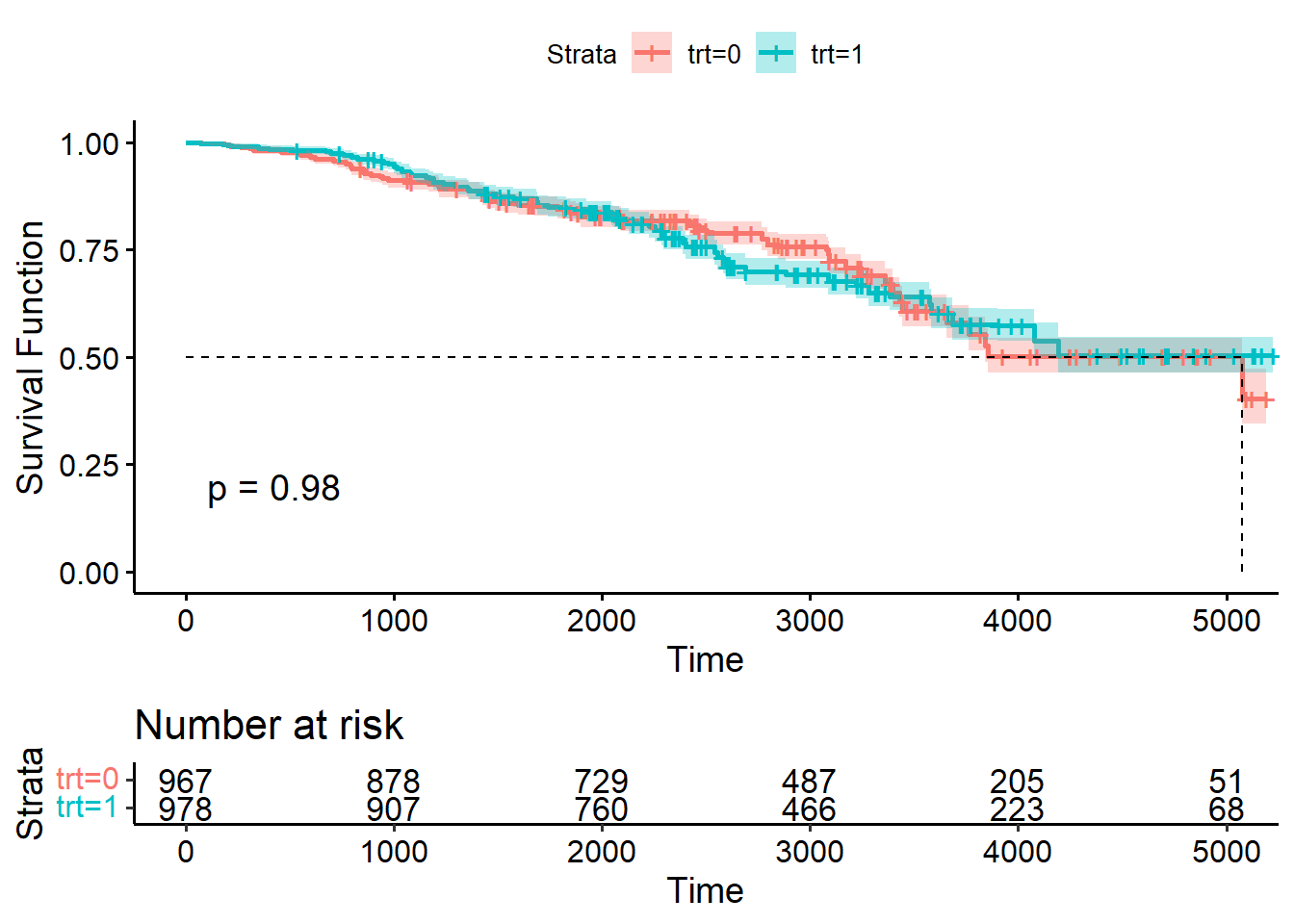
- Step 2: fitting a time-dependent COX PH model on survival status adjusting for trt, age, sex, edema, bili, albumin, ast, and stage with no interaction terms. Make sure categorical variables are fitted as factors.
fit1 <- coxph(Surv(tstart, tstop, status==2) ~ factor(trt) + age + sex + factor(edema) + bili + albumin + ast + factor(stage) , data = pbcseq2)
fit1 %>% tbl_regression(exp=TRUE,
        estimate_fun = partial(style_ratio, digits = 3),
pvalue_fun = partial(style_sigfig, digits = 3))| Characteristic | HR | 95% CI | p-value |
|---|---|---|---|
| factor(trt) | |||
| 0 | — | — | |
| 1 | 0.925 | 0.797, 1.072 | 0.300 |
| age | 1.027 | 1.019, 1.035 | 0.000 |
| sex | |||
| m | — | — | |
| f | 0.541 | 0.447, 0.656 | 0.000 |
| factor(edema) | |||
| 0 | — | — | |
| 0.5 | 1.288 | 1.072, 1.546 | 0.007 |
| 1 | 1.657 | 1.304, 2.106 | 0.000 |
| bili | 1.068 | 1.055, 1.082 | 0.000 |
| albumin | 0.545 | 0.460, 0.647 | 0.000 |
| ast | 1.002 | 1.001, 1.002 | 0.000 |
| factor(stage) | |||
| 1 | — | — | |
| 2 | 0.869 | 0.513, 1.472 | 0.601 |
| 3 | 0.996 | 0.610, 1.627 | 0.988 |
| 4 | 1.164 | 0.715, 1.893 | 0.542 |
| Abbreviations: CI = Confidence Interval, HR = Hazard Ratio | |||
- Step 3: Assess if sex is an effect modifier of trt on survival by adding a sex*trt interaction term and using likelihood ratio test to conclude.
fit2 <- coxph(Surv(tstart, tstop, status==2) ~ factor(trt)*sex + age + factor(edema) + bili + albumin + ast + factor(stage) , data = pbcseq2)
anova(fit2, fit1)
Analysis of Deviance Table
Cox model: response is Surv(tstart, tstop, status == 2)
Model 1: ~ factor(trt) * sex + age + factor(edema) + bili + albumin + ast + factor(stage)
Model 2: ~ factor(trt) + age + sex + factor(edema) + bili + albumin + ast + factor(stage)
loglik Chisq Df Pr(>|Chi|)
1 -3637.7
2 -3637.8 0.1572 1 0.6917- Step 4: Perform model diagnostics
martingaleres <- residuals(fit1, type=c('martingale'))
dfbeta <- residuals(fit1, type=c('dfbeta'))

# marginal residual for continuous variables;
par(mfrow=c(2,2))
# 1. age;
plot(pbcseq2$age, martingaleres, xlab='Age', ylab='Martingale residual')
abline(h=0, lty='dotted')
# 2. bili;
plot(pbcseq2$bili, martingaleres, xlab='bili', ylab='Martingale residual')
abline(h=0, lty='dotted')
# 3. albumin;
plot(pbcseq2$albumin, martingaleres, xlab='albumin', ylab='Martingale residual')
abline(h=0, lty='dotted')
# 4. ast;
plot(pbcseq2$ast, martingaleres, xlab='ast', ylab='Martingale residual')
abline(h=0, lty='dotted')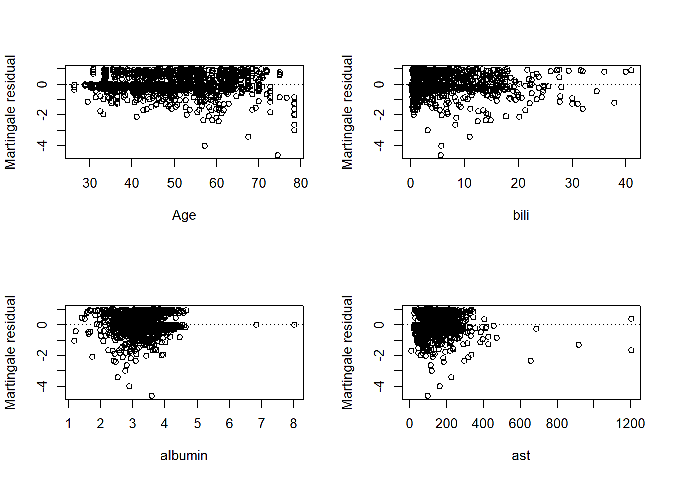
#  Schoenfeld Residuals;
par(mfrow=c(3,3))
cox.zph(fit1, transform="km")
chisq df p
factor(trt) 0.124 1 0.72440
age 4.052 1 0.04413
sex 3.297 1 0.06939
factor(edema) 4.162 2 0.12480
bili 7.350 1 0.00670
albumin 18.897 1 0.000014
ast 0.312 1 0.57636
factor(stage) 14.015 3 0.00288
GLOBAL 37.028 11 0.00011plot(cox.zph(fit1, transform="km"))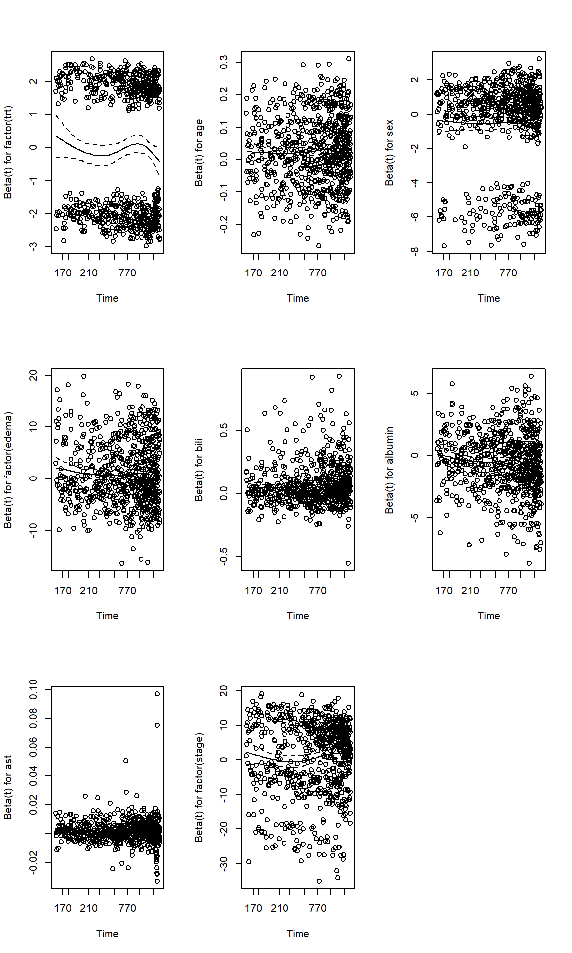
- We identified PH assumption violations. We could potentially try a few things, checking correlation between covariates, estimate HR by time cut-offs etc.
library(corrplot)
## corrplot 0.95 loaded
corrplot(cov2cor(vcov(fit1)))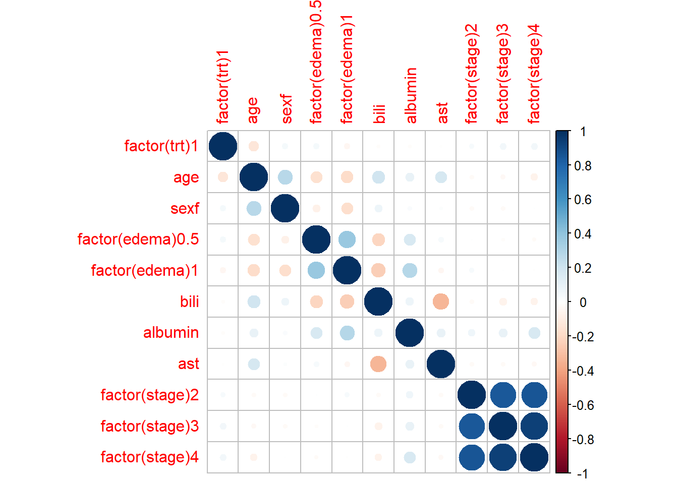
fit3 <- coxph(Surv(tstart, tstop, status==2) ~ factor(trt) + age + sex + factor(edema) + tt(bili) + tt(albumin) + ast + factor(stage), tt = function(x, t, ...) cbind(x*I(t<=2000), x*I(t>2000)), data = pbcseq2)
summary(fit3)
## Call:
## coxph(formula = Surv(tstart, tstop, status == 2) ~ factor(trt) +
##     age + sex + factor(edema) + tt(bili) + tt(albumin) + ast +
##     factor(stage), data = pbcseq2, tt = function(x, t, ...) cbind(x *
##     I(t <= 2000), x * I(t > 2000)))
##
##   n= 1945, number of events= 725
##
##                        coef  exp(coef)   se(coef)      z             Pr(>|z|)
## factor(trt)1     -0.0754115  0.9273618  0.0766147 -0.984             0.324970
## age               0.0265455  1.0269010  0.0039594  6.704    0.000000000020226
## sexf             -0.5982166  0.5497913  0.0984483 -6.076    0.000000001228704
## factor(edema)0.5  0.2395577  1.2706870  0.0937091  2.556             0.010576
## factor(edema)1    0.4574211  1.5799941  0.1250082  3.659             0.000253
## tt(bili)1         0.0663768  1.0686293  0.0072623  9.140 < 0.0000000000000002
## tt(bili)2         0.0800641  1.0833565  0.0113456  7.057    0.000000000001703
## tt(albumin)1     -0.4348759  0.6473450  0.0988714 -4.398    0.000010905207171
## tt(albumin)2     -1.1318166  0.3224470  0.1525234 -7.421    0.000000000000117
## ast               0.0012595  1.0012603  0.0003917  3.215             0.001304
## factor(stage)2   -0.1216686  0.8854418  0.2690434 -0.452             0.651106
## factor(stage)3    0.0227002  1.0229599  0.2502308  0.091             0.927717
## factor(stage)4    0.2016766  1.2234523  0.2487489  0.811             0.417501
##
## factor(trt)1
## age              ***
## sexf             ***
## factor(edema)0.5 *
## factor(edema)1   ***
## tt(bili)1        ***
## tt(bili)2        ***
## tt(albumin)1     ***
## tt(albumin)2     ***
## ast              **
## factor(stage)2
## factor(stage)3
## factor(stage)4
## ---
## Signif. codes:  0 '***' 0.001 '**' 0.01 '*' 0.05 '.' 0.1 ' ' 1
##
##                  exp(coef) exp(-coef) lower .95 upper .95
## factor(trt)1        0.9274     1.0783    0.7981    1.0776
## age                 1.0269     0.9738    1.0190    1.0349
## sexf                0.5498     1.8189    0.4533    0.6668
## factor(edema)0.5    1.2707     0.7870    1.0575    1.5269
## factor(edema)1      1.5800     0.6329    1.2367    2.0187
## tt(bili)1           1.0686     0.9358    1.0535    1.0839
## tt(bili)2           1.0834     0.9231    1.0595    1.1077
## tt(albumin)1        0.6473     1.5448    0.5333    0.7858
## tt(albumin)2        0.3224     3.1013    0.2391    0.4348
## ast                 1.0013     0.9987    1.0005    1.0020
## factor(stage)2      0.8854     1.1294    0.5226    1.5003
## factor(stage)3      1.0230     0.9776    0.6264    1.6705
## factor(stage)4      1.2235     0.8174    0.7514    1.9922
##
## Concordance= 0.721  (se = 0.01 )
## Likelihood ratio test= 535.1  on 13 df,   p=<0.0000000000000002
## Wald test            = 589.5  on 13 df,   p=<0.0000000000000002
## Score (logrank) test = 696.5  on 13 df,   p=<0.0000000000000002
1.3 Model selection
One can use step-wise model select and AIC to finalize the best fitted model. However, there are documented drawbacks of using step-wise, backward, or forward model selection techniques.
- Steyerberg, E.W., Eijkemans, M.J.C. & Habbema, J.D.F. (1999) Stepwise selection in small data sets: a simulation study of bias in logistic regression analysis. Journal of Clinical Epidemiology, 52, 935”942.
Suggest using penalized regression techniques, e.g., LASSO (Least Absolute Shrinkage and Selection Operator), to perform variable selection
- Lasso Regression adds a penalty equal to the absolute value of the magnitude of coefficients to the loss function. e.g., residual sum of squares
- This penalty can shrink some coefficients to exactly zero, effectively performing variable selection.
library(glmnet)
library(MASS)

# 1. using stepwise model selection;
stepAIC(fit1, direction = c("both"), trace = FALSE)
Call:
coxph(formula = Surv(tstart, tstop, status == 2) ~ age + sex +
factor(edema) + bili + albumin + ast + factor(stage), data = pbcseq2)
coef exp(coef) se(coef) z p
age 0.025882 1.026220 0.003928 6.589 0.00000000004414
sexf -0.609055 0.543864 0.097902 -6.221 0.00000000049373
factor(edema)0.5 0.257169 1.293263 0.093198 2.759 0.00579
factor(edema)1 0.499269 1.647516 0.122388 4.079 0.00004515384243
bili 0.065887 1.068106 0.006372 10.341 < 0.0000000000000002
albumin -0.608032 0.544421 0.087211 -6.972 0.00000000000312
ast 0.001501 1.001502 0.000384 3.908 0.00009297472370
factor(stage)2 -0.131861 0.876463 0.268800 -0.491 0.62374
factor(stage)3 0.009541 1.009587 0.249827 0.038 0.96954
factor(stage)4 0.165896 1.180451 0.247952 0.669 0.50345
Likelihood ratio test=515.9 on 10 df, p=< 0.00000000000000022
n= 1945, number of events= 725 # 2. using LASSO;
pbcseq3 <- pbcseq2 %>%
mutate(status2 = case_when(
status == 2 ~ 1,
status %in% c(0,1) ~0
)) %>%
dplyr::select(id, trt, age, sex, edema, bili, albumin, ast, stage, tstart, tstop, status, status2)
x <- model.matrix(fit1)
y <- survival::Surv(pbcseq3$tstart, pbcseq3$tstop, pbcseq3$status2)
library(doParallel)
library(foreach)
cl <- makeCluster(6)
registerDoParallel(cl)
set.seed(123)
cv.fit <- cv.glmnet(x, y, family="cox", alpha=1, parallel = TRUE)
#by cross-validation, we find optimal lambda value that minimizes MSE;
best_lambda <- cv.fit$lambda.min
#we can also use the largest lambda within one standard error of the minimum, leading to a more parsimonious model;
best_lambda2 <- cv.fit$lambda.1se
best_lambda #lambda value that minimizes MSE;[1] 0.00360541best_lambda2 #lambda value within 1 standard error of the minimum;[1] 0.1126949# extract coefficients of from the best model using min lambda;
coef(cv.fit, s = "lambda.min")11 x 1 sparse Matrix of class "dgCMatrix"
1
factor(trt)1 -0.056779736
age 0.024855522
sexf -0.608216230
factor(edema)0.5 0.233295767
factor(edema)1 0.483986870
bili 0.065274647
albumin -0.616513190
ast 0.001399067
factor(stage)2 -0.114025726
factor(stage)3 .
factor(stage)4 0.143898060Interpreting Coefficients from LASSSO:
- Non-zero Coefficients: Variables selected by the model.
- Zero Coefficients: Variables excluded from the model.
- Magnitude and Sign: Indicate the strength and direction of the relationship with the response variable.
#Visualize coefficients across lambda;
#plot of MSE by lambda;
plot(cv.fit, xvar = "lambda", label = TRUE )
abline(v = log(best_lambda), col = "red", lty = 2)
abline(v = log(best_lambda2), col = "blue", lty = 2)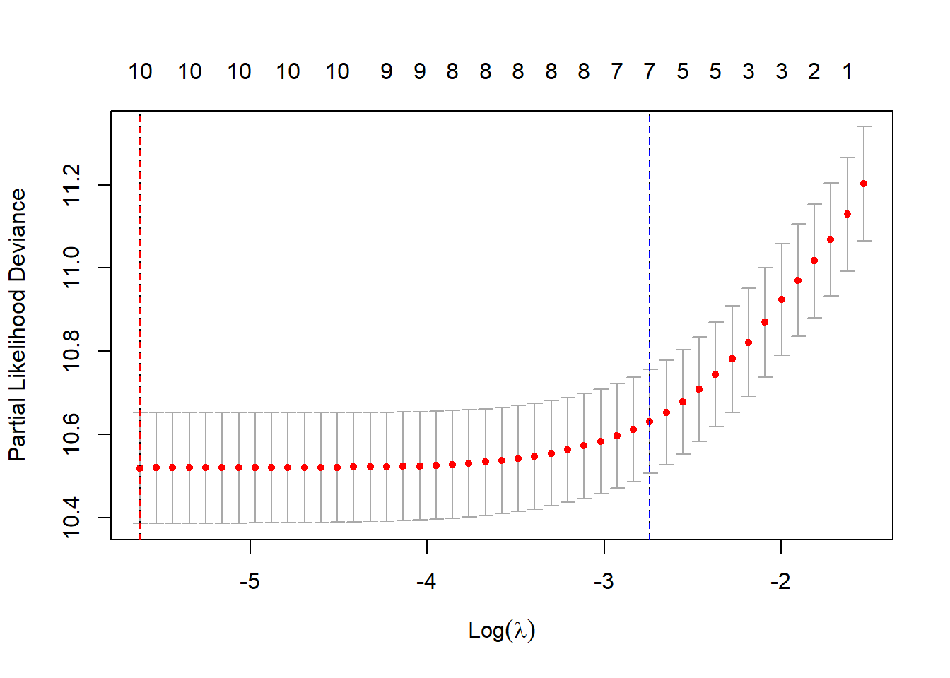
Interpretation:
- Coefficient Paths: Each line represents a coefficient’s path as \(\lambda\) changes.
- Shrinkage: As \(\lambda\) increases (moving left on the log scale), coefficients shrink toward zero.
- Variable Selection: Variables with coefficients that reach zero earlier are less important.
Summary
- From stepwise AIC, 7 variables were selected.
- From LASSO, all 8 variables were selected.
2. Hands-on excecise competing risks
2.1 Liver transplant waiting list
- Subjects on a liver transplant waiting list from 1990-1999, and their disposition: received a transplant, died while waiting, withdrew from the list, or censored.
- Deaths on the liver transplant waiting list: an analysis of competing risks
- Kim WR, Therneau TM, Benson JT, Kremers WK, Rosen CB, Gores GJ, Dickson ER. Deaths on the liver transplant waiting list: an analysis of competing risks. Hepatology. 2006 Feb;43(2):345-51.
A data frame with 815 (transplant) observations on the following 6 variables.
age, age at addition to the waiting list
sex, m or f
abo, blood type: A, B, AB or O
year, year in which they entered the waiting list
futime, time from entry to final disposition
event, final disposition: censored, death, ltx or withdraw
transplant2 <- transplant %>%
  mutate(yeargp = case_when(
    year %in% c(1990,1991,1992) ~ "1990-1992",
    year %in% c(1993,1994,1995) ~ "1993-1995",
    year %in% c(1996,1997) ~ "1996-1997",
    year %in% c(1998,1999) ~ "1998-1999"
  ))

transplant2 %>%
  dplyr::select(-year) %>% #remove year variable from the summary table
  tbl_summary(
  by = yeargp,
  missing_text = "(Missing)") %>%
add_overall()| Characteristic | Overall N = 8151 |
1990-1992 N = 1701 |
1993-1995 N = 2441 |
1996-1997 N = 2101 |
1998-1999 N = 1911 |
|---|---|---|---|---|---|
| age | 52 (44, 58) | 50 (42, 57) | 52 (43, 59) | 51 (43, 58) | 53 (45, 58) |
| (Missing) | 18 | 15 | 3 | 0 | 0 |
| sex | |||||
| m | 447 (55%) | 87 (51%) | 118 (48%) | 125 (60%) | 117 (61%) |
| f | 368 (45%) | 83 (49%) | 126 (52%) | 85 (40%) | 74 (39%) |
| abo | |||||
| A | 325 (40%) | 80 (47%) | 105 (43%) | 68 (32%) | 72 (38%) |
| B | 103 (13%) | 18 (11%) | 33 (14%) | 25 (12%) | 27 (14%) |
| AB | 41 (5.0%) | 8 (4.7%) | 10 (4.1%) | 9 (4.3%) | 14 (7.3%) |
| O | 346 (42%) | 64 (38%) | 96 (39%) | 108 (51%) | 78 (41%) |
| futime | 128 (50, 277) | 41 (18, 83) | 108 (62, 188) | 158 (85, 357) | 318 (153, 516) |
| event | |||||
| censored | 76 (9.3%) | 0 (0%) | 1 (0.4%) | 16 (7.6%) | 59 (31%) |
| death | 66 (8.1%) | 12 (7.1%) | 20 (8.2%) | 18 (8.6%) | 16 (8.4%) |
| ltx | 636 (78%) | 157 (92%) | 205 (84%) | 164 (78%) | 110 (58%) |
| withdraw | 37 (4.5%) | 1 (0.6%) | 18 (7.4%) | 12 (5.7%) | 6 (3.1%) |
| 1 Median (Q1, Q3); n (%) | |||||
# remove data with missing values;
transplant2 <- transplant2[complete.cases(transplant2),]
transplant2$yeargp <- as.factor(transplant2$yeargp)

transplant2$futime[transplant2$futime==0]<-0.01
2.2 Non-parametric analysis using CIF
- Step 1. Generate CIF estimates and use Gray’s test to compare cumulative incidence by blood type. What can you conclude?
library(tidycmprsk)
library(ggsurvfit)
library(cmprsk)

fit1 <- cuminc(ftime = transplant2$futime, fstatus = transplant2$event,
              group = transplant2$abo)

ggcompetingrisks(fit1, palette = "Dark2",
                 legend = "top",
                 ggtheme = theme_bw(),
                 conf.int = TRUE)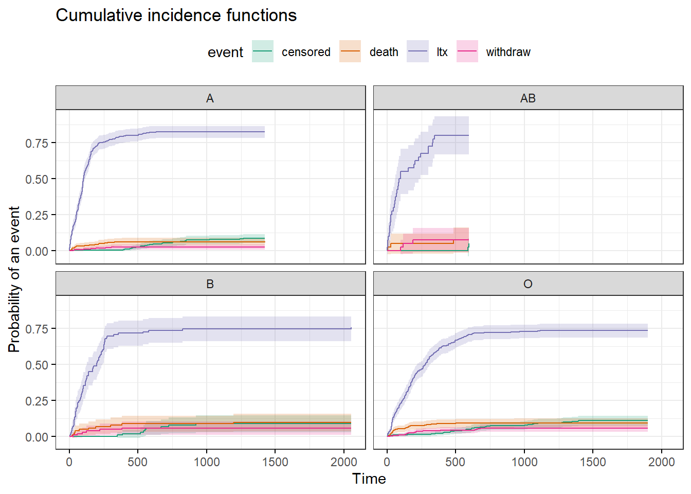
fit2 <- tidycmprsk::cuminc(Surv(futime, event) ~ abo, data = transplant2)
fit2
strata time n.risk estimate std.error 95% CI
A 500 27 0.063 0.014 0.040, 0.094
A 1,000 4 0.063 0.014 0.040, 0.094
A 1,500 0 0.137 0.076 0.032, 0.317
A 2,000 0 0.137 0.076 0.032, 0.317
B 500 12 0.089 0.029 0.043, 0.155
B 1,000 2 0.089 0.029 0.043, 0.155
B 1,500 1 0.128 0.051 0.049, 0.246
B 2,000 1 0.128 0.051 0.049, 0.246
AB 500 2 0.075 0.045 0.017, 0.193
AB 1,000 0 0.075 0.045 0.017, 0.193
AB 1,500 0 0.075 0.045 0.017, 0.193
AB 2,000 0 0.075 0.045 0.017, 0.193
O 500 54 0.093 0.016 0.065, 0.128
O 1,000 14 0.098 0.017 0.069, 0.134
O 1,500 1 0.098 0.017 0.069, 0.134
O 2,000 0 0.098 0.017 0.069, 0.134 strata time n.risk estimate std.error 95% CI
A 500 27 0.805 0.022 0.757, 0.845
A 1,000 4 0.838 0.022 0.789, 0.876
A 1,500 0 0.838 0.022 0.789, 0.876
A 2,000 0 0.838 0.022 0.789, 0.876
B 500 12 0.716 0.045 0.616, 0.794
B 1,000 2 0.773 0.049 0.659, 0.852
B 1,500 1 0.773 0.049 0.659, 0.852
B 2,000 1 0.773 0.049 0.659, 0.852
AB 500 2 0.800 0.067 0.629, 0.898
AB 1,000 0 0.800 0.067 0.629, 0.898
AB 1,500 0 0.800 0.067 0.629, 0.898
AB 2,000 0 0.800 0.067 0.629, 0.898
O 500 54 0.684 0.026 0.630, 0.731
O 1,000 14 0.760 0.025 0.708, 0.804
O 1,500 1 0.776 0.025 0.721, 0.821
O 2,000 0 0.776 0.025 0.721, 0.821 strata time n.risk estimate std.error 95% CI
A 500 27 0.025 0.009 0.012, 0.048
A 1,000 4 0.025 0.009 0.012, 0.048
A 1,500 0 0.025 0.009 0.012, 0.048
A 2,000 0 0.025 0.009 0.012, 0.048
B 500 12 0.059 0.024 0.024, 0.118
B 1,000 2 0.059 0.024 0.024, 0.118
B 1,500 1 0.059 0.024 0.024, 0.118
B 2,000 1 0.059 0.024 0.024, 0.118
AB 500 2 0.075 0.043 0.018, 0.187
AB 1,000 0 0.075 0.043 0.018, 0.187
AB 1,500 0 0.075 0.043 0.018, 0.187
AB 2,000 0 0.075 0.043 0.018, 0.187
O 500 54 0.045 0.011 0.026, 0.071
O 1,000 14 0.066 0.015 0.042, 0.099
O 1,500 1 0.066 0.015 0.042, 0.099
O 2,000 0 0.066 0.015 0.042, 0.099 outcome statistic df p.value
death 1.70 3.00 0.64
ltx 38.6 3.00 <0.001
withdraw 5.71 3.00 0.13 fit2 %>%
ggcuminc(outcome = c("death","ltx","withdraw")) +
ylim(c(0, 1)) +
labs(x = "Days")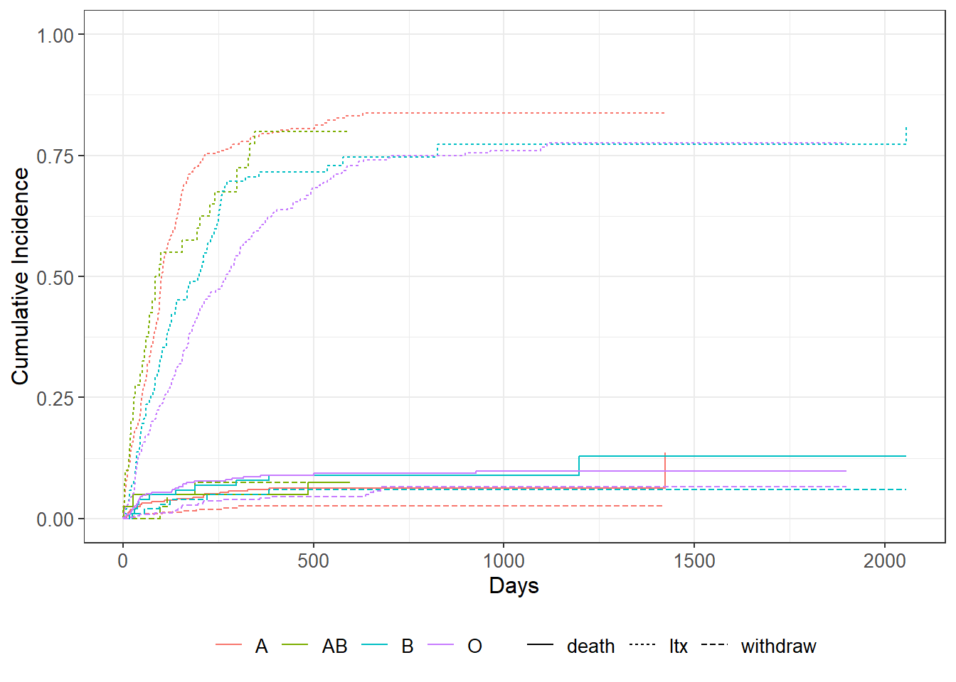
fit3 <- survfit(Surv(futime, event, type = "mstate") ~ abo, data = transplant2)
ggcompetingrisks(fit3, palette = "jco")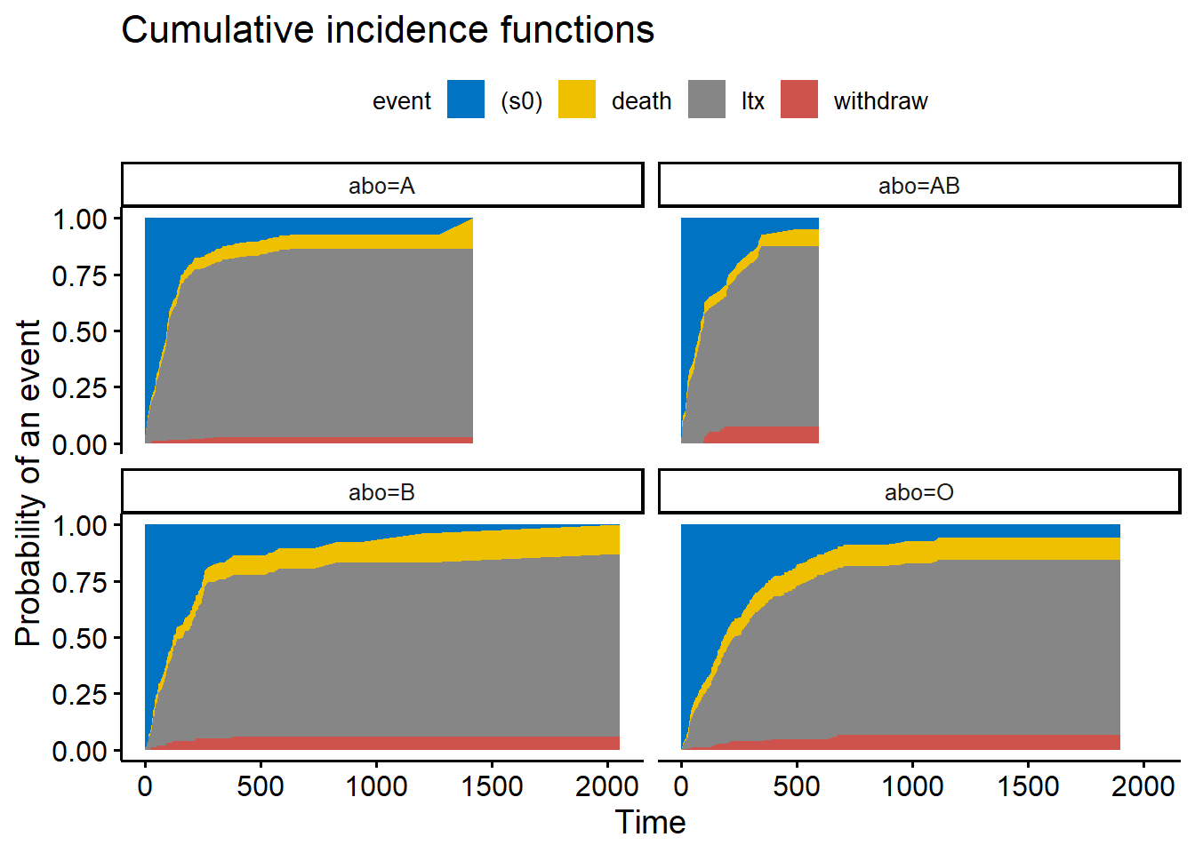
- Step 2. Run step 1 but by variable year group.
2.3 Fitting cause-specific COX PH model on time to transplant (ltx) and time to death (death)
Additive model with no interaction terms: adjusting variable age, sex, abo and year group.
Comment on model results. For example, comparing to the first era, do we observe reduced wait-time in latter entry years?
cox_ltx <- coxph(Surv(futime, event == "ltx")~ age + sex + abo + yeargp, data=transplant2)
summary(cox_ltx)
Call:
coxph(formula = Surv(futime, event == "ltx") ~ age + sex + abo +
yeargp, data = transplant2)
n= 797, number of events= 618
coef exp(coef) se(coef) z Pr(>|z|)
age -0.003195 0.996810 0.004063 -0.786 0.43168
sexf -0.077399 0.925520 0.081669 -0.948 0.34327
aboB -0.347106 0.706730 0.132575 -2.618 0.00884 **
aboAB 0.243886 1.276199 0.188850 1.291 0.19656
aboO -0.641907 0.526288 0.094059 -6.825 0.00000000000882 ***
yeargp1993-1995 -1.202812 0.300348 0.116695 -10.307 < 0.0000000000000002 ***
yeargp1996-1997 -1.752588 0.173325 0.126993 -13.801 < 0.0000000000000002 ***
yeargp1998-1999 -2.596092 0.074564 0.139967 -18.548 < 0.0000000000000002 ***
---
Signif. codes: 0 '***' 0.001 '**' 0.01 '*' 0.05 '.' 0.1 ' ' 1
exp(coef) exp(-coef) lower .95 upper .95
age 0.99681 1.0032 0.98890 1.0048
sexf 0.92552 1.0805 0.78862 1.0862
aboB 0.70673 1.4150 0.54501 0.9164
aboAB 1.27620 0.7836 0.88139 1.8479
aboO 0.52629 1.9001 0.43768 0.6328
yeargp1993-1995 0.30035 3.3295 0.23894 0.3775
yeargp1996-1997 0.17332 5.7695 0.13513 0.2223
yeargp1998-1999 0.07456 13.4112 0.05667 0.0981
Concordance= 0.76 (se = 0.011 )
Likelihood ratio test= 393.9 on 8 df, p=<0.0000000000000002
Wald test = 438.8 on 8 df, p=<0.0000000000000002
Score (logrank) test = 516.7 on 8 df, p=<0.0000000000000002cox_death <- coxph(Surv(futime, event == "death")~ age + sex + abo + yeargp, data=transplant2)
summary(cox_death)Call:
coxph(formula = Surv(futime, event == "death") ~ age + sex +
abo + yeargp, data = transplant2)
n= 797, number of events= 66
coef exp(coef) se(coef) z Pr(>|z|)
age 0.019579 1.019772 0.012988 1.508 0.131679
sexf -0.460495 0.630971 0.258409 -1.782 0.074743 .
aboB 0.162461 1.176402 0.388403 0.418 0.675743
aboAB 0.292653 1.339977 0.619840 0.472 0.636825
aboO 0.007656 1.007685 0.293141 0.026 0.979165
yeargp1993-1995 -0.701524 0.495829 0.377019 -1.861 0.062785 .
yeargp1996-1997 -1.130963 0.322722 0.405960 -2.786 0.005338 **
yeargp1998-1999 -1.451479 0.234224 0.422008 -3.439 0.000583 ***
---
Signif. codes: 0 '***' 0.001 '**' 0.01 '*' 0.05 '.' 0.1 ' ' 1
exp(coef) exp(-coef) lower .95 upper .95
age 1.0198 0.9806 0.9941 1.0461
sexf 0.6310 1.5849 0.3802 1.0471
aboB 1.1764 0.8500 0.5495 2.5186
aboAB 1.3400 0.7463 0.3976 4.5155
aboO 1.0077 0.9924 0.5673 1.7900
yeargp1993-1995 0.4958 2.0168 0.2368 1.0381
yeargp1996-1997 0.3227 3.0986 0.1456 0.7151
yeargp1998-1999 0.2342 4.2694 0.1024 0.5356
Concordance= 0.642 (se = 0.039 )
Likelihood ratio test= 16.29 on 8 df, p=0.04
Wald test = 17.11 on 8 df, p=0.03
Score (logrank) test = 17.97 on 8 df, p=0.022.4 Fitting Fine-Gray model
Additive model with no interaction terms: adjusting variable age, sex, abo and year group.
Comment on model results.
transplant_model <- finegray(Surv(futime, event)~ ., data = transplant2, etype = "ltx")
death_model  <- finegray(Surv(futime, event)~ ., data = transplant2, etype = "death")

fg_ltx <- coxph(Surv(fgstart, fgstop, fgstatus) ~ age + sex + abo + yeargp, data=transplant_model, weight= fgwt)
summary(fg_ltx)
Call:
coxph(formula = Surv(fgstart, fgstop, fgstatus) ~ age + sex +
abo + yeargp, data = transplant_model, weights = fgwt)
n= 3741, number of events= 618
coef exp(coef) se(coef) robust se z
age -0.005313 0.994701 0.003958 0.003425 -1.551
sexf 0.069923 1.072426 0.081754 0.073573 0.950
aboB -0.312875 0.731341 0.131753 0.111473 -2.807
aboAB 0.067040 1.069338 0.189489 0.175616 0.382
aboO -0.540381 0.582526 0.091314 0.079913 -6.762
yeargp1993-1995 -0.987813 0.372390 0.112695 0.111644 -8.848
yeargp1996-1997 -1.212203 0.297541 0.118978 0.115204 -10.522
yeargp1998-1999 -1.855459 0.156381 0.131346 0.132364 -14.018
Pr(>|z|)
age 0.121
sexf 0.342
aboB 0.005 **
aboAB 0.703
aboO 0.0000000000136 ***
yeargp1993-1995 < 0.0000000000000002 ***
yeargp1996-1997 < 0.0000000000000002 ***
yeargp1998-1999 < 0.0000000000000002 ***
---
Signif. codes: 0 '***' 0.001 '**' 0.01 '*' 0.05 '.' 0.1 ' ' 1
exp(coef) exp(-coef) lower .95 upper .95
age 0.9947 1.0053 0.9880 1.0014
sexf 1.0724 0.9325 0.9284 1.2388
aboB 0.7313 1.3674 0.5878 0.9099
aboAB 1.0693 0.9352 0.7579 1.5087
aboO 0.5825 1.7167 0.4981 0.6813
yeargp1993-1995 0.3724 2.6854 0.2992 0.4635
yeargp1996-1997 0.2975 3.3609 0.2374 0.3729
yeargp1998-1999 0.1564 6.3946 0.1206 0.2027
Concordance= 0.726 (se = 0.01 )
Likelihood ratio test= 236.3 on 8 df, p=<0.0000000000000002
Wald test = 230.7 on 8 df, p=<0.0000000000000002
Score (logrank) test = 292.7 on 8 df, p=<0.0000000000000002, Robust = 202.8 p=<0.0000000000000002
(Note: the likelihood ratio and score tests assume independence of
observations within a cluster, the Wald and robust score tests do not).fg_death <- coxph(Surv(fgstart, fgstop, fgstatus) ~ age + sex + abo + yeargp, data=death_model, weight= fgwt)
summary(fg_death)Call:
coxph(formula = Surv(fgstart, fgstop, fgstatus) ~ age + sex +
abo + yeargp, data = death_model, weights = fgwt)
n= 6848, number of events= 66
coef exp(coef) se(coef) robust se z Pr(>|z|)
age 0.01890 1.01908 0.01261 0.01109 1.704 0.0883 .
sexf -0.43181 0.64934 0.25836 0.25583 -1.688 0.0914 .
aboB 0.39298 1.48139 0.38589 0.37007 1.062 0.2883
aboAB 0.14070 1.15108 0.61931 0.62129 0.226 0.8208
aboO 0.39315 1.48164 0.28341 0.27617 1.424 0.1546
yeargp1993-1995 0.04520 1.04623 0.36560 0.35992 0.126 0.9001
yeargp1996-1997 -0.01507 0.98505 0.37635 0.36937 -0.041 0.9675
yeargp1998-1999 -0.01223 0.98784 0.38479 0.37936 -0.032 0.9743
---
Signif. codes: 0 '***' 0.001 '**' 0.01 '*' 0.05 '.' 0.1 ' ' 1
exp(coef) exp(-coef) lower .95 upper .95
age 1.0191 0.9813 0.9972 1.041
sexf 0.6493 1.5400 0.3933 1.072
aboB 1.4814 0.6750 0.7172 3.060
aboAB 1.1511 0.8687 0.3406 3.890
aboO 1.4816 0.6749 0.8623 2.546
yeargp1993-1995 1.0462 0.9558 0.5167 2.118
yeargp1996-1997 0.9850 1.0152 0.4776 2.032
yeargp1998-1999 0.9878 1.0123 0.4697 2.078
Concordance= 0.595 (se = 0.033 )
Likelihood ratio test= 7.2 on 8 df, p=0.5
Wald test = 8.69 on 8 df, p=0.4
Score (logrank) test = 6.99 on 8 df, p=0.5, Robust = 8.56 p=0.4
(Note: the likelihood ratio and score tests assume independence of
observations within a cluster, the Wald and robust score tests do not).2.5 Comparing cause-specific COX PH model and Fine-Gray model
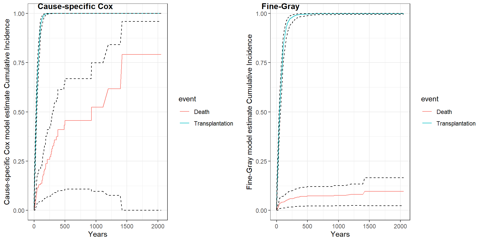
Step 1: comment on the estimated coefficients and associated significant between the two approaches.
step 2: compare model estimated CIF
CIF.cox <- data.frame(
    CIF = c(1- survfit(cox_ltx)$surv,1- survfit(cox_death)$surv),
    CIF_l = c(1- survfit(cox_ltx)$upper,1- survfit(cox_death)$upper),
    CIF_u = c(1- survfit(cox_ltx)$lower,1- survfit(cox_death)$lower),
    time = c(survfit(cox_ltx)$time,survfit(cox_death)$time),
    event = c(rep("Transplantation", length(survfit(cox_ltx)$time)),
              rep("Death", length(survfit(cox_death)$time))))

p1<-CIF.cox %>%
    ggplot( aes(x=time, y=CIF, group=event, color=event)) +
    geom_line()+
    geom_line(aes(x=time, y=CIF_l), color="black", linetype = "dashed")+
    geom_line(aes(x=time, y=CIF_u), color="black", linetype = "dashed")+
    ylim(0,1)+
    xlab("Years")+
    ylab("Cause-specific Cox model estimate Cumulative Incidence")+
    theme_bw()

CIF.fg <- data.frame(
    CIF = c(1- survfit(fg_ltx)$surv,1- survfit(fg_death)$surv),
    CIF_l = c(1- survfit(fg_ltx)$upper,1- survfit(fg_death)$upper),
    CIF_u = c(1- survfit(fg_ltx)$lower,1- survfit(fg_death)$lower),
    time = c(survfit(fg_ltx)$time,survfit(fg_death)$time),
    event = c(rep("Transplantation", length(survfit(fg_ltx)$time)),
              rep("Death", length(survfit(fg_death)$time))))

p2<-CIF.fg %>%
    ggplot(aes(x=time, y=CIF, group=event, color=event)) +
    geom_line()+
    geom_line(aes(x=time, y=CIF_l), color="black", linetype = "dashed")+
    geom_line(aes(x=time, y=CIF_u), color="black", linetype = "dashed")+
    ylim(0,1)+
    xlab("Years")+
    ylab("Fine-Gray model estimate Cumulative Incidence")+
    theme_bw()

library(cowplot)
plot_grid(p1, p2, labels = c('Cause-specific Cox', 'Fine-Gray'), label_size = 12)