A competing risk is an event whose occurrence precludes the occurrence of the primary event of interest.
violating the non-informative censoring assumption in conventional Cox PH modelling.
e.g., In a study in which the primary outcome was time to ICU death, ICU discharge in this case would be an competing event, precluding the occurrence of the primary event.
A competing risks analysis should appropriately incorporating the competing event into the analysis.
Patients are still at risk to experience other outcomes!
Analysis that treats other events as random censoring, or considers time to the first occurred outcome will lead to bias analysis.
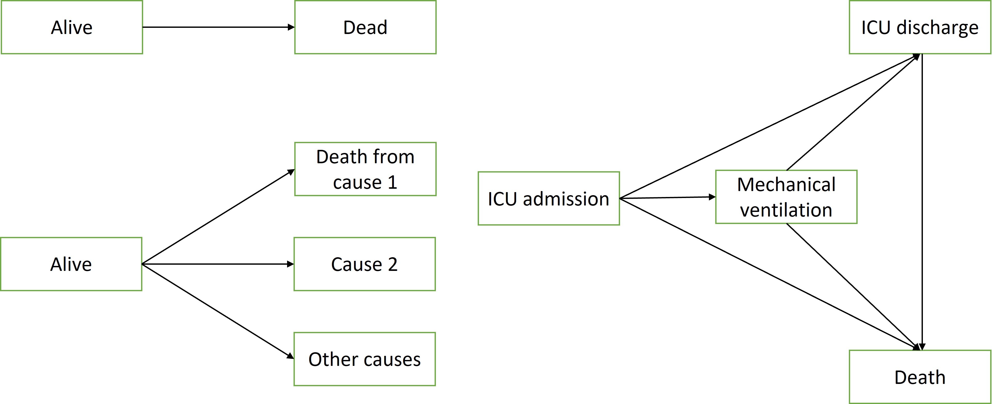
1. Competing risks can be viewed as a multi-state survival problem
Three example multi-state models.
The upper left is a simple survival diagram,
we can view death as an absorbing state
the lower left is an example of competing risks,
and the lower right panel is a multi-state illness-death model.
In application, there are 5 steps proposed by Staffa and Zurakowski (2019) to design and analyze a competing risks study
determine whether competing risks analysis is needed (do you have informative censoring?)
perform nonparametric analysis first
perform a model-based analysis
interpret results
comparing to traditional survival analysis, this may not be necessary but will help you understand the impact of competing events
2. The “incorrect” Naive analysis
Understanding the issues of the naive approach can provide insight into the competing risks program and statistical methods to appropriately handle competing risks
Naive analysis: modelling death from other causes (status=2) as censoring, by folding the competing risk into a two-status outcome, where we no longer need to distinguish between event types
the Kaplan-Meier estimator takes the patients who are censored to still be at risk, i.e., they will go on to experience the event
However, of course those who experienced the competing risk are not ‘still at risk’, results in the estimated survivor function being under estimated; over-estimate event rates!
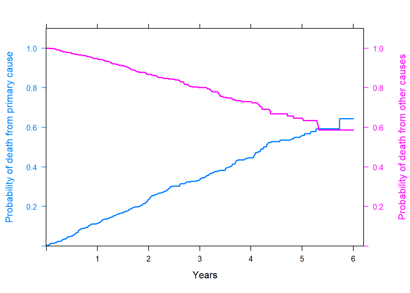
# incorrect KM estimates;library(tidyverse)library(survminer)library(survival)library(latticeExtra)fit_incorrect1 <-survfit(Surv(time, status==1)~1, data=fourD)fit_incorrect2 <-survfit(Surv(time, status==2)~1, data=fourD)surv.km <- fit_incorrect1$survtime.km <- fit_incorrect1$timesurv.other.km <- fit_incorrect2$survcumDist.km =1-surv.km #cumulative incidence distribution;km_primary <-xyplot(cumDist.km ~ time.km, type ="l",lwd=2, ylim =c(0,1.1), xlim =c(0,6.2), ylab ="Probability of death from primary cause", xlab ="Years")km_other <-xyplot(surv.other.km ~ time.km, type ="l" , lwd=2, ylim =c(0,1.1), ylab ="Probability of death from other causes")doubleYScale(km_primary, km_other, add.ylab2 =TRUE, use.style=T)
Figure shows that the two curves cross.
At 5 years, the probability of dying of primary cause is 0.44, and of other causes it is 0.64. The sum of the two probabilities exceed 1 - over estimate event rates!
Nonparametric estimation using cumulative incidence functions (CIF)
1. Connection between CIF, suvival and hazard functions
In the absence of competing risks, the cumulative incidence function is equivalent to the cumulative distribution function
the probability or risk of an event occurring by time \(t\).
CIF and hazard function is related! Thus, if a covariate is associate with change in the rate of which events occur, we can also conclude that it will be associate with cahnges in the probability of the event occuring.
The direction of the association will be concordant between analysis based on CIF and the hazard function.
2. Cause-specific CIF
The probability of experiencing an event by time \(t\) and that the event experience is of type \(j\), \(j = 1, \ldots, J\) and \(D \in \{1, \ldots, J\}\) be the event type indicator.
\[
CIF_j(t) = Pr(T \leq t, D = j)
\]
\[
\lim_{t \rightarrow \infty} CIF_j(t) < 1
\]
as time goes to infinity, in the presence of competing event, the probability of experiencing event type j will be less than 100%
“referred to as a subdistribution function”
Using KM estimator of \(CIF_j(t)\) will result in under estimated survival as we have shown before.
Several estimators do not exhibit this bias has been proposed
Alen-Johansen estimator for CIF
standard error of the AJ estimator can be computed using jackknife or bootstrap technique
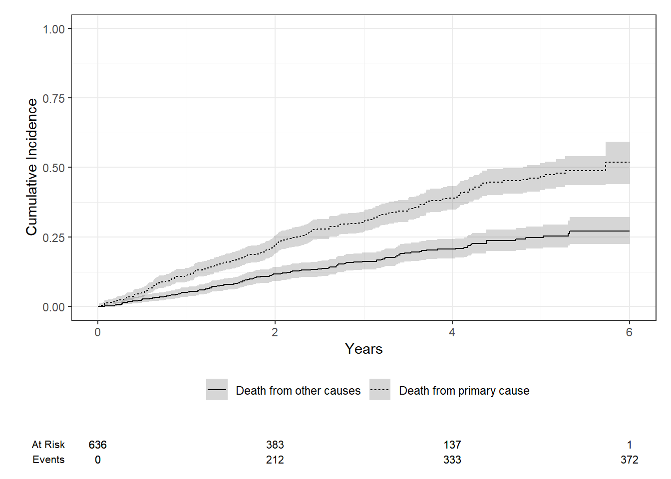
in R we can use cuminc() function under the tidycomprsk package to calculate CIF.
we can use Gray’s test, a modified Chi-squared test, to compare CIF between 2 or more groups (similar to the log-rank test).
library(tidycmprsk)library(ggsurvfit)# change status to a factor;fourD$status2 <-as.factor(fourD$status)levels(fourD$status2) <-c("Censored", "Death from primary cause", "Death from other causes")fit1 <-cuminc(Surv(time, status2) ~1, data = fourD)fit1
fit1 %>%ggcuminc(outcome =c("Death from primary cause", "Death from other causes")) +ylim(c(0, 1)) +labs(x ="Years")+add_confidence_interval() +add_risktable()
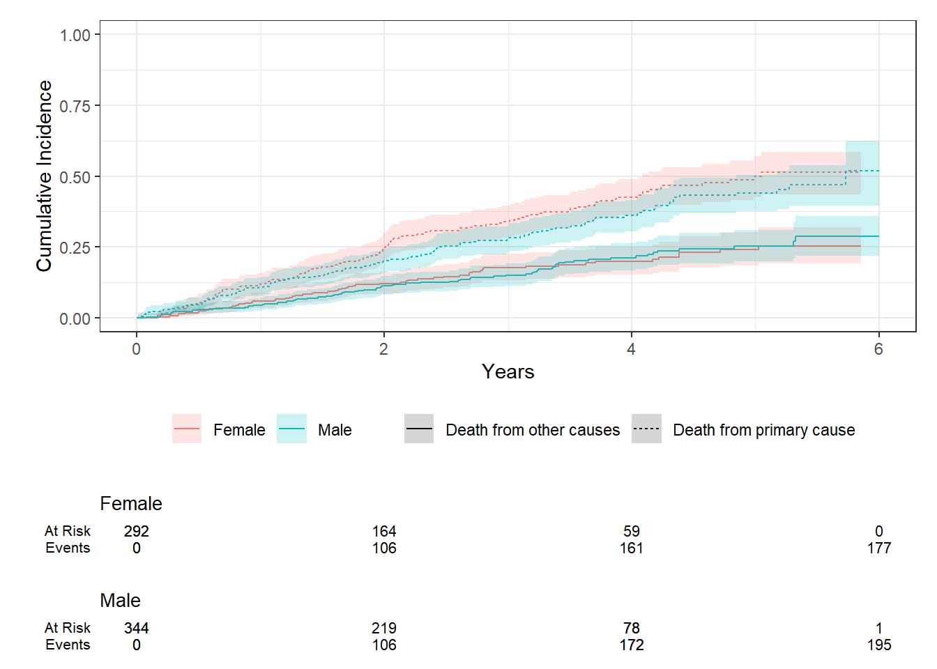
Suppose we want to compare cause-specific CIF by sex, we can use Gray’s test.
fit2 <-cuminc(Surv(time, status2) ~ sex, data = fourD)fit2
outcome                    statistic   df     p.value
Death from primary cause   2.06        1.00   0.15
Death from other causes    0.011       1.00   0.91
fit2 %>%ggcuminc(outcome =c("Death from primary cause", "Death from other causes")) +ylim(c(0, 1)) +labs(x ="Years")+add_confidence_interval() +add_risktable()
fit2 %>%tbl_cuminc(times =c(1,5), outcome =c("Death from primary cause", "Death from other causes"),label_header ="**Year {time}**") %>%add_p()
instantaneous rate of occurrence of the given type of event in subjects who are currently event-free
redefining the failure indicator to be 1 if and only if the patient fails due specifically to cause \(j\)
estimated using Cox regression
Subdistribution hazards
instantaneous rate of occurrence of the given type of event in subjects who have not yet experienced an event of that type
estimated using Fine-Gray regression
Assumptions
independent observations
in the presence of correlated data, we can fit a cluster or frailty term on the cause-specific hazard model and the Fine-Gray model
Non-informative censoring
Proportional hazard assumption
We have to check for PH assumption for both approaches!
use cox.zph() to test for association between hazard and time
2. Difference between the two approaches
Cause-specific Cox model
an individual is removed from the risk set when a failure due to other causes occurs
the interpretation of the regression coefficients relates to the cause-specific hazard function.
intuitive interpretation on both direct and magnitude of the effect on the hazard rate.
Fine-Gray model
the individual remains in the risk set for cause \(j\) when a failure due to other causes occurs
The interpretation of the regression coefficients relates to the subdistribution hazard function
be cautious of your interpretation! Comment on effect direction (e.g., variable x increases the risk of outcome), but not the magnitude. Austin and Fine (2017)
When to use which approach?
suggest to use the Fine-Gray subdistribution hazard model when the focus is on estimating incidence or predicting prognosis in the presence of competing risks.
suggest to use the cause-specific hazard model when the focus is on addressing etiologic questions
3. Cause-specific Cox PH Model
we can fit cause-specific Cox PH model easily using coxph() function - from lecture 3.
if your data contains two competing events, you will fit two cause-specific Cox model for each event.
same approaches to perform model diagnostics!
# cause 1 Cox model;fit3_1 <-coxph(Surv(time, status ==1) ~ age + sex, data = fourD)fit3_1 %>%tbl_regression(exp =TRUE)
Characteristic
HR
95% CI
p-value
age
1.02
1.00, 1.04
0.016
sex
Female
—
—
Male
0.88
0.68, 1.14
0.3
Abbreviations: CI = Confidence Interval, HR = Hazard Ratio
# cause 2 cox model;fit3_2 <-coxph(Surv(time, status ==2) ~ age + sex, data = fourD)fit3_2 %>%tbl_regression(exp =TRUE)
Characteristic
HR
95% CI
p-value
age
1.07
1.04, 1.09
<0.001
sex
Female
—
—
Male
1.19
0.84, 1.69
0.3
Abbreviations: CI = Confidence Interval, HR = Hazard Ratio
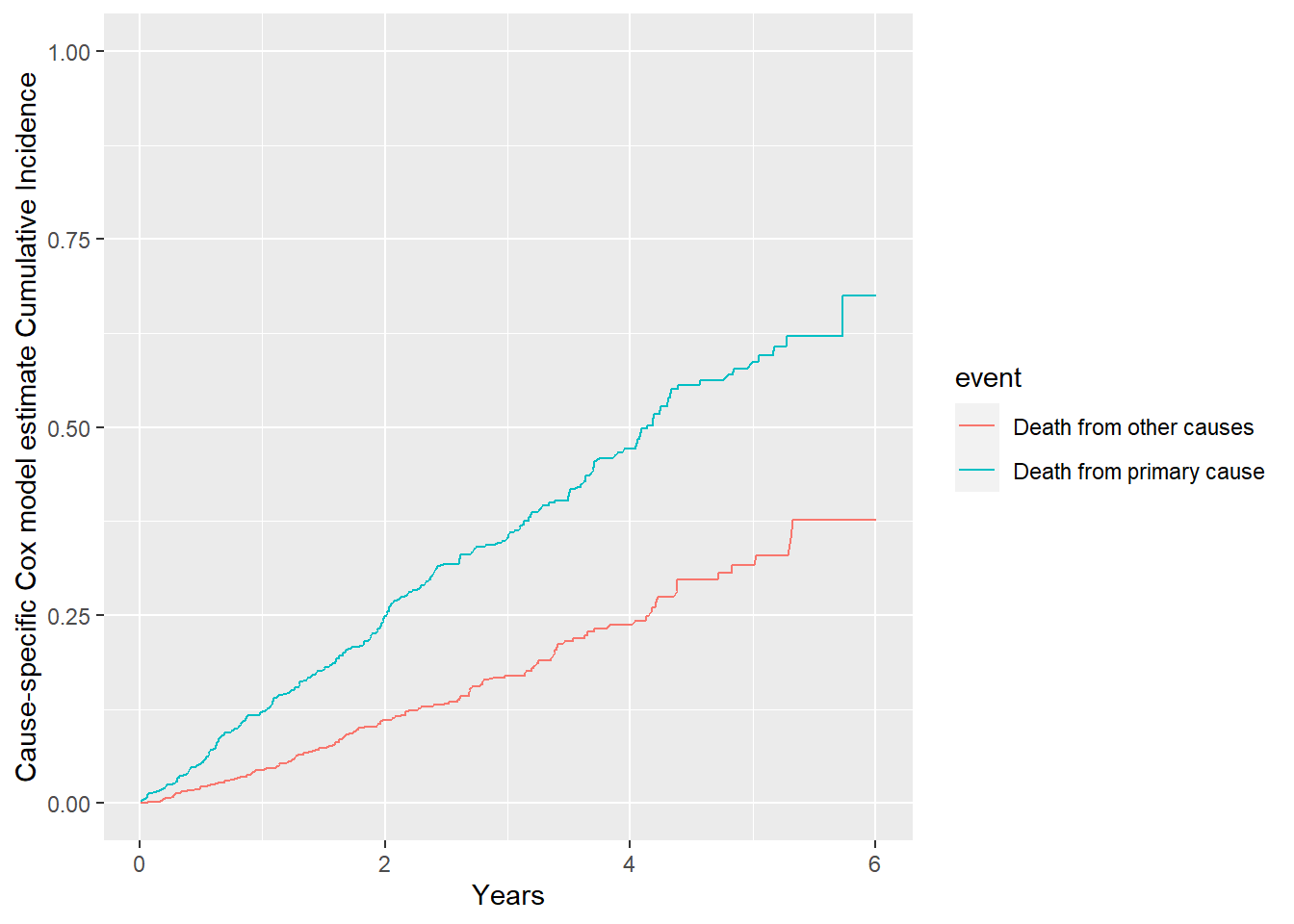
# model estimated CIF;# it's possible to add in confidence interval using confidence interval of the estimated survival;CIF.cox <-data.frame(CIF =c(1-survfit(fit3_1)$surv,1-survfit(fit3_2)$surv),time =c(survfit(fit3_1)$time,survfit(fit3_2)$time),event =c(rep("Death from primary cause", length(survfit(fit3_1)$time)), rep("Death from other causes", length(survfit(fit3_2)$time))))CIF.cox %>%ggplot( aes(x=time, y=CIF, group=event, color=event)) +geom_line()+ylim(0,1)+xlab("Years")+ylab("Cause-specific Cox model estimate Cumulative Incidence")
# checking for PH assumption;cox.zph(fit3_1)
        chisq df    p
age    0.9441  1 0.33
sex    0.0729  1 0.79
GLOBAL 0.9454  2 0.62
cox.zph(fit3_2)
       chisq df    p
age    1.871  1 0.17
sex    0.778  1 0.38
GLOBAL 3.342  2 0.19
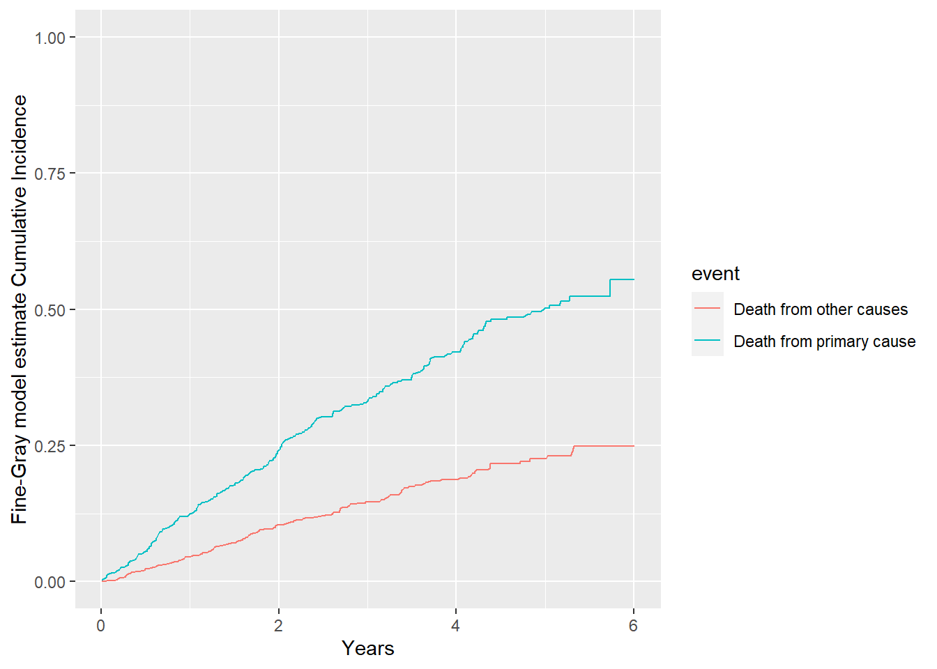
4. Fine-Gray subdistribution hazards model
primary <-finegray(Surv(time, as.factor(status))~ age + sex, data = fourD,etype ="1")other <-finegray(Surv(time, as.factor(status))~ age + sex, data = fourD,etype ="2")#creating fine-gray weights;head(primary)
  age    sex fgstart    fgstop fgstatus fgwt
1  60   Male       0 5.8480493        0    1
2  68 Female       0 5.2539357        0    1
3  70 Female       0 2.9541410        1    1
4  69   Male       0 0.9856263        1    1
5  58 Female       0 0.2902122        1    1
6  63   Male       0 3.9452430        1    1
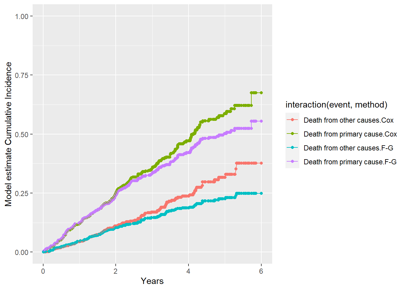
More on difference between the two modelling approaches for completing risks
Difference on Hazard function specification
The cause-specific hazard function focuses on the risk of experiencing the event of interest, assuming the individual has not yet experienced either the event of interest or any competing event.
Mathematically, for cause \(k\), the cause-specific hazard at time \(t\) is defined as:
\[ \lambda_k(t \mid X) = \lim_{\Delta t \to 0} \frac{\Pr(t \leq T < t + \Delta t, \text{event is of type } k \mid T \geq t, X)}{\Delta t}\]
Where:
\(T\) is the time to the event.
\(X\) is a vector of covariates.
\(\lambda_k(t \mid X)\) is the instantaneous risk of experiencing event \(k\) at time \(t\), given that no event (neither the event of interest nor any competing event) has occurred before time \(t\).
The subdistribution hazard from Fine-Gray for cause \(k\) is given by:
\[
\lambda_k^{sub}(t \mid X) = \lim_{\Delta t \to 0} \frac{\Pr(t \leq T < t + \Delta t, \text{event is of type } k \mid T \geq t \text{ or competing event by time } t, X)}{\Delta t}
\]
This differs from the cause-specific hazard because:
The risk set for the subdistribution hazard includes individuals who have already experienced competing events (but with modified risks), while the risk set for the cause-specific hazard excludes them once a competing event occurs.
The subdistribution hazard directly models the cumulative incidence function (CIF), which gives the probability of an event happening over time, considering the possibility of competing events.
Difference on Risk Set Defitniions
Cause-specific hazard: The risk set only includes individuals who are event-free for both the event of interest and competing events up to time \(t\).
\[
\mathcal{R}(t) = \{ i : T_i \geq t \}
\]
Subdistribution hazard: The risk set includes individuals who are either event-free or have experienced a competing event by time \(t\). The Fine-Gray model retains individuals who experienced competing events in the risk set by adjusting their contribution.
\[
\mathcal{R}^{sub}(t) = \{ i : T_i \geq t \text{ or competing event by time } t \}
\]
Difference on CIF
Cause-specific hazard: The cumulative incidence for cause \(k\), denoted as \(F_k(t)\), can be derived from the cause-specific hazard function using the following relationship:
\[
F_k(t) = \int_0^t \lambda_k(s) S(s) \, ds
\]
where \(S(t)\) is the overall survival function (the probability of no event occurring by time \(t\)).
Subdistribution hazard: In the Fine-Gray model, the subdistribution hazard directly governs the cumulative incidence function for the event of interest. The cumulative incidence function can be written as:
Cause-specific hazard ratios describe the effect of covariates on the instantaneous risk of the event of interest, conditional on being event-free up to time (t).
Subdistribution hazard ratios describe the effect of covariates on the cumulative incidence of the event of interest, accounting for competing risks.
Main points
Misinterpretation of Hazard Ratios:
The hazard ratio in the Fine-Gray model corresponds to the subdistribution hazard of an event, which is different from the cause-specific hazard (which reflects the instantaneous risk of an event given that no competing event has occurred).
Interpreting these hazard ratios as affecting the absolute risk of an event can be misleading because the Fine-Gray hazard ratios are conditional on survival up to time \(t\) without experiencing a competing event. Hence, they do not directly measure the effect of covariates on the probability of the event of interest occurring.
The Fine-Gray model links covariates to the cumulative incidence function, which gives the probability of an event over time. While this is the prepered approach for predicting absolute risks, the hazard ratios derived from this model do not correspond to the instantaneous risk but rather how covariates shift the entire cumulative risk.
Recommendations for Analyzing Competing Risk Survival Data, Austin et al (2016)
(Non-parametric/univariate) Cumulative incidence functions (CIFs) should be used to estimate the incidence of each of the different types of competing risks.
Do not use the Kaplan-Meier estimate of the survival function for this purpose.
Researchers need to decide whether the research objective is on addressing etiologic questions or on estimating incidence or predicting prognosis.
etiologic, cause-specific cox PH model
incidence estimation/prediction, Fine-Gray subdistribution hazard model
In some settings, both types of regression models should be estimated for each of the competing risks to permit a full understanding of the effect of covariates on the incidence and the rate of occurrence of each outcome.
Be careful of how you interpret coefficients from the Fine-Gray model
the covariates can be concluded as having an effect on the CIF (the probabiltiy/risk of experiencing event \(j\)).
However, it is important to note that magnitude of the subdistribution hazard ratio does not
This interpretation error appears to frequently in the medical literature.
Proportional hazard assumption is needed for both approaches! Model diagnostic and validation are key steps.