The hazard ratio compares instantaneous risks among those who have already survived to time \(t\). Because treatment can change who survives up to \(t\), the sets being compared are post-treatment selected, so the hazard ratio generally lacks a simple causal interpretation even with no unmeasured confounding.
Let \(T^{(a)}\) denote the potential event time under treatment \(a\in\{0,1\}\). The (cause-specific) hazard under \(a\) is \[
\lambda_a(t)
= \lim_{\Delta t \downarrow 0}
\frac{\Pr\{t \le T^{(a)} < t+\Delta t \mid T^{(a)} \ge t\}}{\Delta t},
\] and the (time-specific) hazard ratio is \[
\mathrm{HR}(t) \;=\; \frac{\lambda_1(t)}{\lambda_0(t)}.
\]
Two issues make \(\mathrm{HR}(t)\) non-causal:
Conditioning on a post-treatment variable. The risk set at time \(t\) is those with \(T^{(a)}\!\ge t\). If treatment affects early survival, then \[
\{T^{(1)} \ge t\} \;\text{and}\; \{T^{(0)} \ge t\}
\] include different compositions of individuals because of treatment itself. Thus, even if \((T^{(0)},T^{(1)}) \perp A \mid L\) (no unmeasured confounding given \(L\)), the event \(\{T^{(a)}\ge t\}\) is not independent of \(A\). Comparing \(\lambda_1(t)\) vs \(\lambda_0(t)\) is therefore a comparison of selected subpopulations at time \(t\), not a clean “effect of treatment on outcome.”
Non-collapsibility. Even without confounding, marginal and conditional hazard ratios differ: \[
\frac{\lambda_1(t)}{\lambda_0(t)}
\;\neq\;
\sum_{\ell} w_\ell \,\frac{\lambda_1(t\mid L=\ell)}{\lambda_0(t\mid L=\ell)} ,
\] so the hazard ratio does not aggregate to a population-average causal contrast. One can observe \(\mathrm{HR}(t)\!\approx\!1\) while survival probabilities differ meaningfully across arms.
Survival Probability Causal Effect
A more transparent target is the survival probability causal effect (often called SPCE): \[
\Delta_S(t) \;=\; S_1(t) - S_0(t),
\qquad
S_a(t) \;=\; \Pr\{T^{(a)} > t\}.
\]
\(\Delta_S(t)\) is a collapsible - the difference in the probability of being event-free at time \(t\) if everyone were treated vs if everyone were untreated. - We can compute \(\Delta_S(t)\) using propensity score weighted Kaplan-Meier estimation. - Extensions is possible to incorporate informative censoring and competing risks.
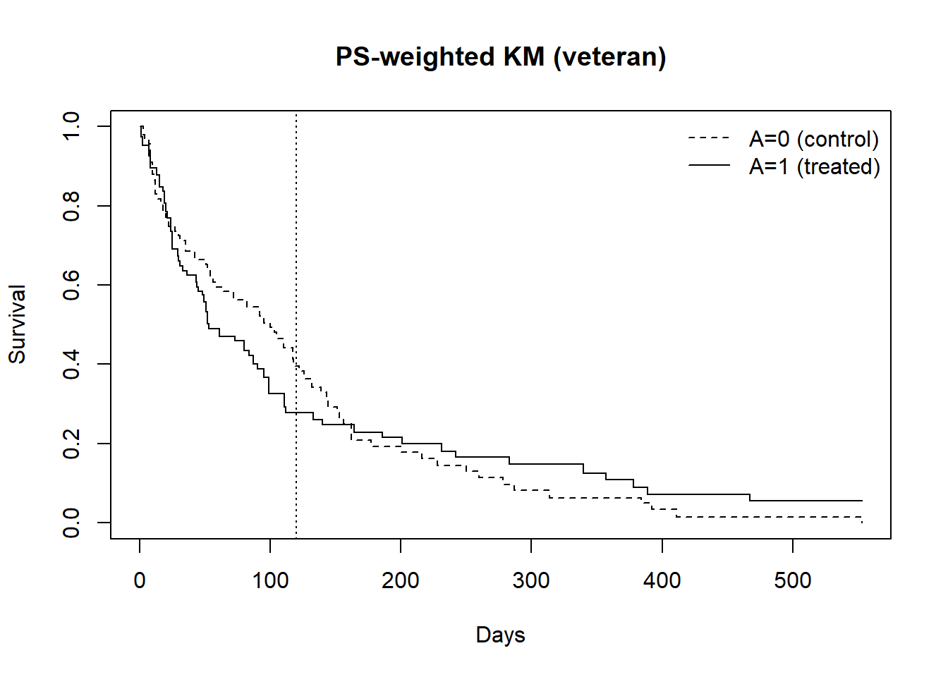
1. Hands on tutorial 1 on fitting PS-weighted marginal Cox and PS-weighted KM.
Mathematically, we will aim at estimating SPCE. - the survival probability causal effect (SPCE) at a chosen time \(t\), i.e. \[
\Delta_S(t) \equiv S_1(t) - S_0(t)
\] where \(S_a(t)=Pr\{T^{(a)}>t\}\) is the counterfactual survival probability under treatment \(a, a\in \{0,1\}\).
Causal assumptions:
Stable unit treatmnet assumption (no multiple versions of treatment and no interference)
Consistency (i.e., observed outcome is consistent with their potential outcome under the treatment they actually received),
Positivity (i.e., non-zero probability of receiving any of the treatment levels),
Conditional exchangeability (also known as no unmeasured confounding).
1.5 Bootstrap confidence interval for causal estimand
set.seed(123)n <-nrow(dat1) #sample size;B <-1000#bootstrap iterations;boot_SPCE <-numeric(B)for (b in1:B) {# Resample subjects with replacement idx <-sample.int(n, size = n, replace =TRUE) bdat <- dat1[idx, ]# fit PS and recompute stabilized IPTW (ATE) IPTWb <-weightit(A ~ age + karno + diagtime + prior + celltype,data = bdat, method ="glm", #using the default logistic regression;stabilize =TRUE,estimand ="ATE") bdat$w <- IPTWb$weights fitA1_b <-survfit(Surv(time, event) ~1, data =subset(bdat, A==1),weights = bdat$w[bdat$A==1]) fitA0_b <-survfit(Surv(time, event) ~1, data =subset(bdat, A==0),weights = bdat$w[bdat$A==0]) S1_b <-as.numeric(summary(fitA1_b, times = t_star, extend =TRUE)$surv) S0_b <-as.numeric(summary(fitA0_b, times = t_star, extend =TRUE)$surv) boot_SPCE[b] <- S1_b - S0_b}# Percentile 95% CIsquantile(boot_SPCE, c(0.025, 0.975))
       2.5%       97.5%
-0.26620470  0.03855422
1.6 “Causal” Hazard ratio (not causally interpretable!)
cox1 <-coxph(Surv(time, event) ~ A, data = dat1, weights = w, robust =TRUE)summary(cox1)
2. Hands on tutorial on causal survival analysis with a competing event.
We now consider competing risks where the event of interest is death and the competing event is liver transplant. Let \(A\in\{0,1\}\) and in a competing-risk setting let the outcome of interest be death and the competing event be transplant.
For treatment option, the cumulative incidence function (CIF) for death is \[
F_a^{\text{death}}(t)=\Pr\{T_a \le t,\ \text{cause}=\text{death}\}.
\] We target the absolute risk difference between treated and untreated as our causal esitmand of interest. \[
\Delta_F(t)=F_1^{\text{death}}(t)-F_0^{\text{death}}(t).
\]
There are two weighting strategies for causal competing risk analysis
we have a competing event and censoring is considered non-informative)
Use IPTW to reweight the sample to the ATE target and then compute a weighted Aalen-Johansen estimator of the CIF. If administrative censoring is non-informative and independent of covariates, we do not need to estimate the censoring process or weight by censoring under this approach.
Alternatively, we can consider applying censoring weights and combine censoring weights with treatmet weights (e.g., IPTW + IPCW; continuous-time censoring model under informative censoring process).
Construct time-specific risk estimators that require IPCW and propose a continuous-time censoring model (e.g., Cox) to estimate time-specific plug-in estimator for the CIF of each event (primary and competing) under treated and control.
Take away
If you believe administrative censoring is non-informative and independent of covariates, use IPTW weighted AJ estimator.
If censoring may depend on \(A\) and/or \(L\), use IPTW x IPCW (continuous time censoring model). We will leave this out for this tutorial.
Conditional exchangeability (no unmeasured confounding)
Positivity on treatment and censoring where \(\Pr\{C^*_a > t\} > 0\) over the time.
Independent censoring given the model used for IPCW
2.1 Reaching data - Revisit the Mayo Clinic Primary Biliary Cirrhosis
An analysis based on the data can be found in Murtagh, et. al. (1994)
Murtaugh PA. Dickson ER. Van Dam GM. Malinchoc M. Grambsch PM. Langworthy AL. Gips CH. “Primary biliary cirrhosis: prediction of short-term survival based on repeated patient visits.” Hepatology. 20(1.1):126-34, 1994.
id: case number
age: in years
sex: m/f
trt: 1/2/NA for D-penicillmain, placebo, not randomized
time: number of days between registration and the earlier of death,
transplantation, or study analysis in July, 1986
status: status at endpoint, 0/1/2 for censored, transplant, dead
day: number of days between enrolment and this visit date
all measurements below refer to this date
albumin: serum albumin (mg/dl)
alk.phos: alkaline phosphotase (U/liter)
ascites: presence of ascites
ast: aspartate aminotransferase, once called SGOT (U/ml)
bili: serum bilirunbin (mg/dl)
chol: serum cholesterol (mg/dl)
copper: urine copper (ug/day)
edema: 0 no edema, 0.5 untreated or successfully treated 1 edema despite diuretic therapy
hepato: presence of hepatomegaly or enlarged liver
platelet: platelet count
protime: standardised blood clotting time
spiders: blood vessel malformations in the skin
stage: histologic stage of disease (needs biopsy)
trig: triglycerides (mg/dl)
In this data, patients are censored at the time of transplantation. The data do not follow patients who received transplant.
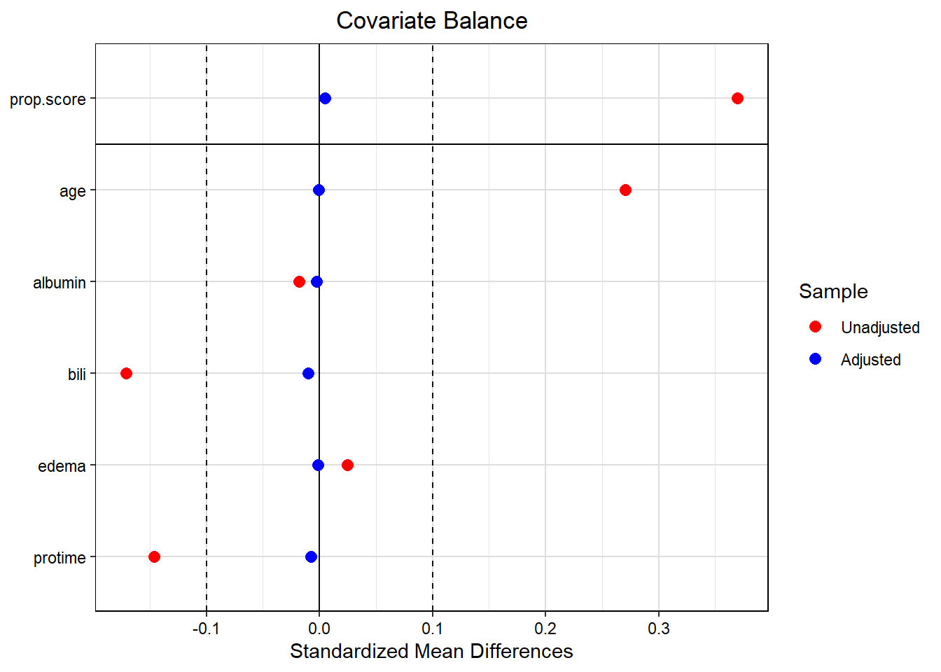
dat2$w<-IPTW$weights # adding PS weights back to the data;
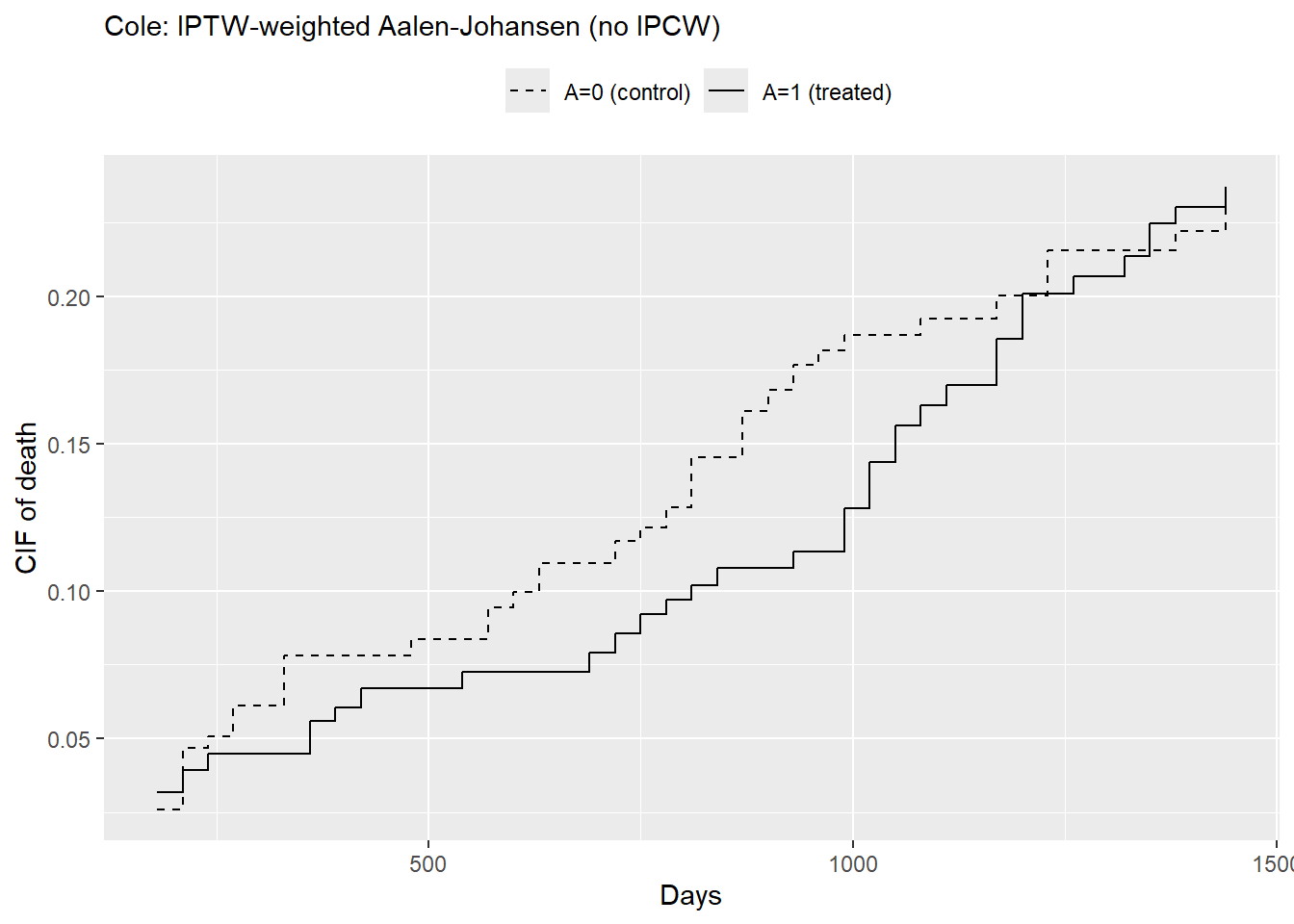
2.4 Weighted AJ estimator with transplant as the competing event under administrative, non-informative censoring
# we do not consider censoring weights under the assumption of non-informative censoring;library(prodlim)fit_cif_AJ <-prodlim(Hist(time, status) ~ A,data = dat2,caseweights = dat2$w)# Time horizont_star <-365*2# 2 yearsF1_AJ <-predict(fit_cif_AJ, cause =2, times = t_star,newdata =data.frame(A =1))F0_AJ <-predict(fit_cif_AJ, cause =2, times = t_star,newdata =data.frame(A =0))RD_AJ <- F1_AJ - F0_AJRD_AJ
[1] -0.03139891
# cause-specific CIFts <-seq(180, 180*8, by=30)F1_curve <-predict(fit_cif_AJ, cause =2, times = ts, newdata =data.frame(A=1))F0_curve <-predict(fit_cif_AJ, cause =2, times = ts, newdata =data.frame(A=0))df_AJ <-data.frame(t=ts, F1=F1_curve, F0=F0_curve, dF=F1_curve-F0_curve)ggplot(df_AJ, aes(x = t)) +geom_step(aes(y = F0, color ="A=0 (control)", linetype ="A=0 (control)")) +geom_step(aes(y = F1, color ="A=1 (treated)", linetype ="A=1 (treated)")) +scale_color_manual(name ="",values =c("A=0 (control)"="black", "A=1 (treated)"="black") ) +scale_linetype_manual(name ="",values =c("A=0 (control)"="dashed", "A=1 (treated)"="solid") ) +labs(x ="Days",y ="CIF of death",title ="Cole: IPTW-weighted Aalen-Johansen (no IPCW)" ) +theme(plot.title =element_text(size =11),legend.position ="top")
2.5 Adding Bootstrap confidence interval
set.seed(123)n <-nrow(dat2) #sample size;B <-1000#bootstrap iterations;boot_wCIF <-numeric(B)for (b in1:B) {# Resample subjects with replacement idx <-sample.int(n, size = n, replace =TRUE) bdat <- dat2[idx, ]# fit PS and recompute stabilized IPTW (ATE) IPTWb <-weightit(A ~ age + albumin + bili + edema + protime,data = bdat, method ="glm",stabilize =TRUE,estimand ="ATE") bdat$w <- IPTWb$weights fit_cif_AJ <-prodlim(Hist(time, status) ~ A, data = bdat, caseweights = bdat$w) t_star <-365*2# 2 years F1_AJ <-predict(fit_cif_AJ, cause =2, times = t_star,newdata =data.frame(A =1)) F0_AJ <-predict(fit_cif_AJ, cause =2, times = t_star,newdata =data.frame(A =0)) RD_AJ <- F1_AJ - F0_AJ boot_wCIF[b] <- F1_AJ - F0_AJ}# Percentile 95% CIsquantile(boot_wCIF, c(0.025, 0.975))# 2.5% 97.5% # -0.08819970 0.02251391