Days from registration to death, transplantation, or study analysis (July 1986)
days
trt
Treatment assignment
1 = D-penicillamine; 2 = placebo; NA = not randomized
trig
Triglycerides
mg/dL
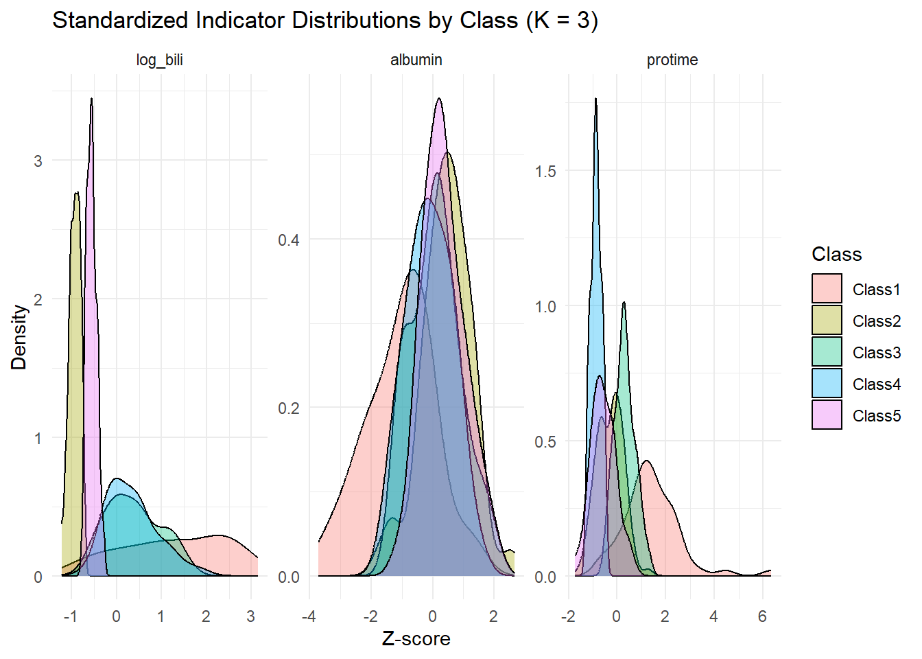
We use three continuous lab measures (bili, albumin, protime). We apply a log transform to bilirubin to reduce skew, then standardize all indicators to zero mean and unit variance for interpretability in profile plots.
library(mclust)library(survival)library(tidyverse)library(forcats)library(survminer)library(gtsummary)set.seed(123)needed_vars <-c("time","status","age_years","sex","trt","edema","ascites","hepato","spiders","bili","albumin","protime")dat <- survival::pbc %>%as_tibble() %>%transmute( id, time, status, death =as.integer(status ==2),age_years = age /365.25, sex, trt, edema, ascites, hepato, spiders, bili, albumin, protime ) %>% tidyr::drop_na(dplyr::all_of(needed_vars)) %>%mutate(log_bili =log1p(bili))# Standardized continuous indicators for LPA (continuous-only)X <-scale(dat[, c("log_bili", "albumin", "protime")])head(dat)
# A tibble: 6 × 15
     id  time status death age_years sex     trt edema ascites hepato spiders
  <int> <int>  <int> <int>     <dbl> <fct> <int> <dbl>   <int>  <int>   <int>
1     1   400      2     1     0.161 f         1   1         1      1       1
2     2  4500      0     0     0.155 f         1   0         0      1       1
3     3  1012      2     1     0.192 m         1   0.5       0      0       0
4     4  1925      2     1     0.150 f         1   0.5       0      1       1
5     5  1504      1     0     0.104 f         2   0         0      1       1
6     6  2503      2     1     0.181 f         2   0         0      1       0
# ℹ 4 more variables: bili <dbl>, albumin <dbl>, protime <dbl>, log_bili <dbl>
LPA/LCA assumes that, conditional on class, indicators follow a multivariate normal distribution with class-specific means and covariance structure.
Consider candidate number of clusters from 2 clusters to 5 clusters
Best model is determined by
Primary: largest BIC
Supported by higher entropy and larger posterior membership probability;
Posterior class membership probabilities (per subject): For each individual, the model gives a vector of probabilities-one for each class (e.g., Person A: 0.72 in Class 1, 0.25 in Class 2, 0.03 in Class 3).
Entropy:takes all those individual probability vectors and boils them down to one summary number that reflects how concentrated they are on average.
Ks <-2:5fits <-vector("list", length(Ks))names(fits) <-as.character(Ks)entropy_norm <-function(Z) { p <-pmax(as.matrix(Z), .Machine$double.eps) N <-nrow(p); K <-ncol(p)-sum(p *log(p)) / (N *log(K)) # [0,1], higher = crisper}metrics <-lapply(Ks, function(K){ fitK <-Mclust(X, G = K) # lets mclust choose best covariance for this K fits[[as.character(K)]] <<- fitK post <- fitK$ztibble(K = K,BIC = fitK$bic,Entropy =entropy_norm(post),AvgMaxPost =mean(apply(post, 1, max)) )}) %>%bind_rows()metrics