Group-based trajectory modelling

1. Hands-on example of fitting a group-based trajectory model

This tutorial aims to provide a quick example for implementing flexmix R package to run a group-based trajectory model.

1.1 The ICTUS (Impact of Cholinergic Treatment USe) cohort

• Design: Prospective, multicenter longitudinal observational cohort of Alzheimer’s disease (AD) patients in Europe

  • A cohort of 1380 patients with Alzheimer disease followed-up in 12 European countries.

  • These patients were included between February 2003 and July 2005 in 29 centres specialized in neurology, geriatrics, psychiatry, or psycho-geriatrics with a recognized experience in the diagnosis and management of Alzheimer disease.

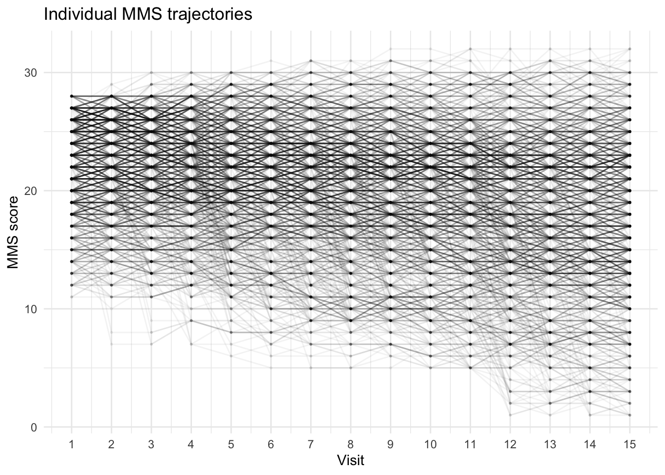
  • These patients were examined at six-month intervals over two years. Each examination included (though not exclusively) an Mini Mental Score (MMS) assessment.

• Recruitment period: 2003–2005

• Study aims including to describe natural history and clinical course of mild–moderate AD

• Reynish, E., Cortes, F., Andrieu, S., Cantet, C., Olde Rikkert, M., Melis, R., Froelich, L., Frisoni, G., Jonsson, L., Visser, P., et al., 2007. The ictus study: A prospective longitudinal observational study of 1,380 ad patients in europe. Neuroepidemiology 29 (1-2), 29-38

• Vellas, B., Hausner, L., Frolich, L., Cantet, C., Gardette, V., Reynish, E., Gillette, S., Aguera-Morales, E., Auriacombe, S., Boada, M., et al., 2012. Progression of alzheimer disease in europe: Data from the european ictus study. Current Alzheimer Research 9 (8), 902-912.

library(tidyverse)
library(DT)

ictusShort <- read.csv("ictusShort.csv", header = TRUE)

# look at new data;
datatable(ictusShort,
          rownames = FALSE,
          options = list(dom = 't')) 

str(ictusShort)

'data.frame':   1374 obs. of  16 variables:
 $ id    : chr  "I-1" "I-2" "I-3" "I-4" ...
 $ MMS.1 : int  18 22 26 19 22 20 15 26 24 23 ...
 $ MMS.2 : int  17 20 26 20 22 20 15 27 25 24 ...
 $ MMS.3 : int  16 22 26 19 21 19 13 26 25 23 ...
 $ MMS.4 : int  16 20 25 20 23 18 10 25 23 25 ...
 $ MMS.5 : int  16 20 28 19 21 20 11 24 21 22 ...
 $ MMS.6 : int  17 19 27 18 23 20 9 26 21 22 ...
 $ MMS.7 : int  17 21 27 19 23 20 7 22 23 21 ...
 $ MMS.8 : int  17 21 26 20 21 21 7 23 21 20 ...
 $ MMS.9 : int  17 20 27 18 21 17 7 22 22 21 ...
 $ MMS.10: int  18 20 26 19 22 17 6 24 22 19 ...
 $ MMS.11: int  18 21 27 18 22 20 5 25 21 18 ...
 $ MMS.12: int  17 14 27 19 22 21 5 23 22 17 ...
 $ MMS.13: int  15 12 27 17 20 21 7 23 23 16 ...
 $ MMS.14: int  13 12 29 16 22 21 3 24 22 16 ...
 $ MMS.15: int  14 14 28 16 22 7 5 23 23 17 ...

1.2 Descriptive analysis

library(gtsummary)
library(stringr)

# reshape to long: one row per person per visit
ictus_long <- ictusShort %>%
  pivot_longer(
    cols = starts_with("MMS."),
    names_to = "visit_raw",
    values_to = "MMS"
  ) %>%
  mutate(
    # extract the integer after "MMS."
    visit = as.integer(str_extract(visit_raw, "\\d+"))
  ) %>%
  select(id, visit, MMS) %>%
  arrange(id, visit)

mms_summary_by_visit <- ictus_long %>%
  group_by(visit) %>%
  summarise(
    n          = sum(!is.na(MMS)),
    mean_MMS   = mean(MMS, na.rm = TRUE),
    sd_MMS     = sd(MMS, na.rm = TRUE),
    median_MMS = median(MMS, na.rm = TRUE),
    p25_MMS    = quantile(MMS, 0.25, na.rm = TRUE),
    p75_MMS    = quantile(MMS, 0.75, na.rm = TRUE),
    .groups    = "drop"
  ) %>%
  mutate(
    across(
      c(mean_MMS, sd_MMS, median_MMS, p25_MMS, p75_MMS),
      ~ round(.x, 1)
    )
  )

datatable(
  mms_summary_by_visit,
  rownames = FALSE,
  options = list(dom = "t", pageLength = 15)
)

ictus_long %>%
  ggplot(aes(x = visit, y = MMS, group = id)) +
  geom_line(alpha = 0.05) +
  geom_point(alpha = 0.05, size = 0.4) +
  scale_x_continuous(breaks = 1:15) +
  labs(
    x = "Visit",
    y = "MMS score",
    title = "Individual MMS trajectories"
  ) +
  theme_minimal()

1.3 Group-based trajectory modelling with flexmix R package

Model 1 Three classes

library(flexmix)

set.seed(123)

# 3-class model
mod3 <- flexmix(
  MMS ~ poly(visit, 2, raw = TRUE) | id,
  data = ictus_long,
  k = 3,
  control = list(minprior=0) # by default flexmix drop a class if miniprior threshold less than 0.05;
)

# BIC for 3-class
BIC(mod3)

[1] 103097.3

Model 2 Four classes

set.seed(123)

mod4 <- flexmix(
  MMS ~ poly(visit, 2, raw = TRUE) | id,
  data = ictus_long,
  k = 4,
  control = list(minprior=0)
)

BIC(mod4)

[1] 98081.2

Model 3 Five classes

set.seed(123)

mod5 <- flexmix(
  MMS ~ poly(visit, 2, raw = TRUE) | id,
  data = ictus_long,
  k = 5,
  control = list(minprior=0)
)

BIC(mod5)

[1] 96094.5

Compare models

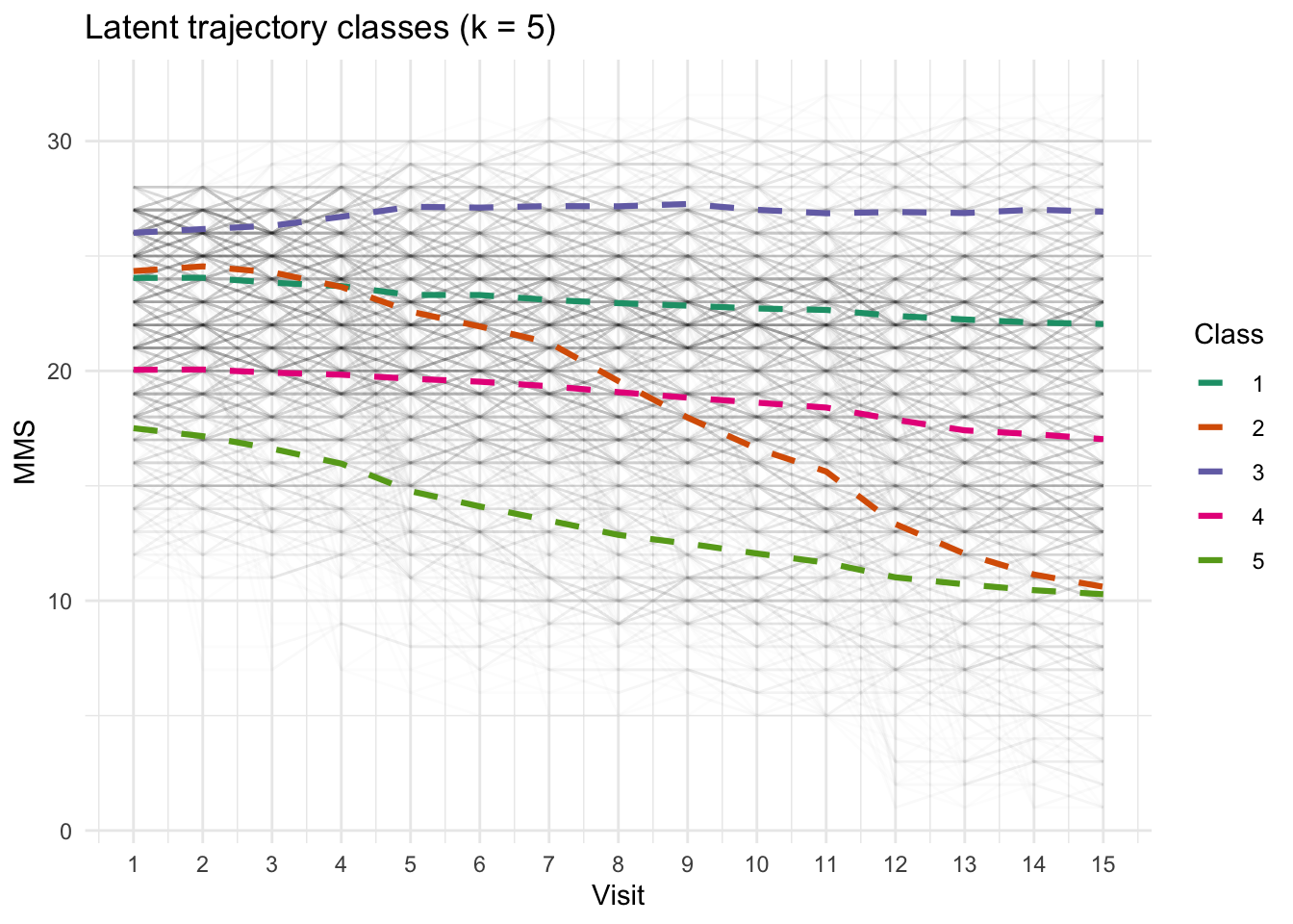
# comparing BIC (lower better);
# Five clusters best model;
bic_comp <- tibble(
  k   = c(3, 4, 5),
  BIC = c(BIC(mod3), BIC(mod4), BIC(mod5))
)

bic_comp

# A tibble: 3 × 2
      k     BIC
  <dbl>   <dbl>
1     3 103097.
2     4  98081.
3     5  96095.

# we can also compare using likelihood ratio test Lo–Mendell–Rubin test;
library(tidyLPA)
# LMR for k vs k–1 needs the k–1 model, so we add a 2-class model
mod2 <- flexmix(
  MMS ~ poly(visit, 2, raw = TRUE) | id,
  data = ictus_long,
  k = 2
)

BIC(mod2)

[1] 110131

# log-likelihoods
ll2 <- as.numeric(logLik(mod2))
ll3 <- as.numeric(logLik(mod3))
ll4 <- as.numeric(logLik(mod4))
ll5 <- as.numeric(logLik(mod5))

# number of parameters (flexmix stores this in attr(logLik, "df"))
p2 <- attr(logLik(mod2), "df")
p3 <- attr(logLik(mod3), "df")
p4 <- attr(logLik(mod4), "df")
p5 <- attr(logLik(mod5), "df")

# 2-class (null) vs 3-class (alt)
lmr_2_vs_3 <- calc_lrt(
  n            = 1374,
  null_ll      = ll2,
  null_param   = p2,
  null_classes = 2,
  alt_ll       = ll3,
  alt_param    = p3,
  alt_classes  = 3
)

lmr_2_vs_3

Lo-Mendell-Rubin ad-hoc adjusted likelihood ratio rest:

LR = 7083.361, LMR LR (df = 5) = 6770.995, p < 0.001

# 3-class (null) vs 4-class (alt)
lmr_3_vs_4 <- calc_lrt(
  n            = 1374,
  null_ll      = ll3,
  null_param   = p3,
  null_classes = 3,
  alt_ll       = ll4,
  alt_param    = p4,
  alt_classes  = 4
)

lmr_3_vs_4

Lo-Mendell-Rubin ad-hoc adjusted likelihood ratio rest:

LR = 5065.769, LMR LR (df = 5) = 4842.375, p < 0.001

# 4-class (null) vs 5-class (alt)
lmr_4_vs_5 <- calc_lrt(
  n            = 1374,
  null_ll      = ll4,
  null_param   = p4,
  null_classes = 4,
  alt_ll       = ll5,
  alt_param    = p5,
  alt_classes  = 5
)

lmr_4_vs_5

Lo-Mendell-Rubin ad-hoc adjusted likelihood ratio rest:

LR = 2036.369, LMR LR (df = 5) = 1946.568, p < 0.001

Final model: five classes

# assess class certainty;
# For everyone assigned to class k, what is the mean posterior probability of that class?;

post5_mat <- posterior(mod5)
head(post5_mat)

             [,1]         [,2]          [,3]      [,4]       [,5]
[1,] 4.427551e-38 0.0004083933 4.856156e-116 0.9297276 0.06986404
[2,] 4.427551e-38 0.0004083933 4.856156e-116 0.9297276 0.06986404
[3,] 4.427551e-38 0.0004083933 4.856156e-116 0.9297276 0.06986404
[4,] 4.427551e-38 0.0004083933 4.856156e-116 0.9297276 0.06986404
[5,] 4.427551e-38 0.0004083933 4.856156e-116 0.9297276 0.06986404
[6,] 4.427551e-38 0.0004083933 4.856156e-116 0.9297276 0.06986404

# hard class label for each row by highest proability;
class_vec <- clusters(mod5)   

# posterior probability *for the assigned class* for each row
assigned_prob <- post5_mat[cbind(seq_len(nrow(post5_mat)), class_vec)]

# mean posterior for assigned class by class
mean_assigned_by_class <- tapply(assigned_prob, class_vec, mean)
mean_assigned_by_class

        1         2         3         4         5 
0.9852494 0.9835952 0.9860250 0.9811287 0.9822495 

ictus_long5 <- ictus_long %>%
  mutate(class5 = factor(clusters(mod5)))

n_per_class <- ictus_long5 %>%
  distinct(id, class5) %>%
  count(class5, name = "n_patients")

n_per_class

# A tibble: 5 × 2
  class5 n_patients
  <fct>       <int>
1 1             427
2 2             122
3 3             198
4 4             341
5 5             286

mms_class_mean <- ictus_long5 %>%
  group_by(class5, visit) %>%
  summarise(
    mean_MMS = mean(MMS, na.rm = TRUE),
    .groups  = "drop"
  )

ggplot() +
  # raw spaghetti in faint black
  geom_line(
    data  = ictus_long5,
    aes(x = visit, y = MMS, group = id),
    color = "black",
    alpha = 0.01
  ) +
  # mean trajectories per class as dashed coloured lines
  geom_line(
    data  = mms_class_mean,
    aes(x = visit, y = mean_MMS, color = class5),
    linetype = "dashed",
    size = 1.1
  ) +
  scale_x_continuous(breaks = 1:15) +
  scale_color_brewer(palette = "Dark2") +
  labs(
    x = "Visit",
    y = "MMS",
    color = "Class",
    title = "Latent trajectory classes (k = 5)"
  ) +
  theme_minimal()