My first class on Bayesian inference - Conjugate prior

Learning Objectives

• Learn two simple Bayesian models (Beta-binomial & normal-normal)
• Discuss practical advantages and disadvantages of Bayesian approach

1. Introduction to Bayesian approach

The Bayesian approach to parameter estimation is based on Bayes’ theorem.

Let \(\theta\) be the parameter of interest and \(y\) be the observed data.

\[\begin{aligned} P(\theta \mid y) & = \frac{P(y \mid \theta)P(\theta)}{P(y)} \\ & = \frac{\text{likelihood of the data given the parameter} \times \text{prior}}{\text{marginal distribution of the data}} \\ & \propto \text{likelihood}(y \mid \theta ) \times \text{prior}(\theta) \end{aligned}\]

• \(P(y)\) is called a normalizing constant. It ensures that \(\int P(\theta \mid y)\, d\theta = 1\), so that the posterior distribution is a proper probability distribution.

• Its numerical value is usually not of direct interest, unless we are comparing different models for the data.

• The key idea in Bayes’ theorem is that the posterior distribution is proportional to the likelihood times the prior: \[P(\theta \mid y) \propto P(y\mid \theta)P(\theta).\]

Likelihood vs probability distribution

• Probability distribution: a function of the data when the parameter is fixed.
  • A probability distribution \(f(y\mid \theta)\) sums or integrates to 1 over all possible values of the random variable \(Y\), with \(\theta\) treated as fixed.
  • It answers the question: “If the parameter were \(\theta\), how likely is each possible outcome \(y\)?”
• Likelihood: the same mathematical expression, but viewed as a function of the parameter when the observed data are fixed.
  • The likelihood function is written as \(L(\theta \mid y_{obs}) \propto f(y_{obs}\mid \theta)\).
  • It answers the question: “Given the observed data \(y_{obs}\), which values of \(\theta\) are more plausible?”
  • A likelihood does not need to integrate to 1 over \(\theta\). In the likelihood, the data are fixed and \(\theta\) varies.

Bayes’ Rule

The ELISA test for HIV was widely used in the mid-1990s for screening blood donations. Like most medical diagnostic tests, ELISA is not perfect.

• If a person truly carries the HIV virus, experts estimated that the test gives a positive result 97.7% of the time. This is the sensitivity of the test.
• If a person does not carry the HIV virus, ELISA gives a negative result 92.6% of the time. This is the specificity of the test.
• Suppose the HIV prevalence in the population at that time was 0.5%. This is the prior base rate.

Now suppose a randomly selected individual tests positive. We want the conditional probability that the person truly carries HIV.

• We know the probability of a positive test if HIV is truly present: \[P(T^+ \mid D^+) = 0.977,\]
• and the probability of a positive test if HIV is not present: \[P(T^+ \mid D^-) = 1 - 0.926 = 0.074.\]

Using Bayes’ rule, we can obtain the posterior probability of disease given a positive test result:

\[\begin{aligned} P(D^+ \mid T^+) & = \frac{P(T^+ \mid D^+)P(D^+)}{P(T^+)} \\ & = \frac{P(T^+ \mid D^+)P(D^+)}{P(T^+ \mid D^+)P(D^+) + P(T^+ \mid D^-)P(D^-)}. \end{aligned}\]

This is a simple example of Bayesian updating: we start with a prior probability of disease and update it using the observed test result.

Mathematically,

\[\begin{aligned} P(D^+ \mid T^+) & = \frac{P(D^+ \text{ and } T^+)}{P(T^+)}\\ & = \frac{P(T^+ \mid D^+)P(D^+)}{P(T^+)} \\ & = \frac{P(T^+ \mid D^+)P(D^+)}{P(T^+ \mid D^+)P(D^+) + P(T^+ \mid D^-)P(D^-)} \\ & = \frac{0.977 \times 0.005}{0.977 \times 0.005 + 0.074 \times 0.995} \\ & = \frac{0.0049}{0.0785} = 0.0622. \end{aligned}\]

So even after a positive test result, the probability that the person truly has HIV is only about 6.2%, because the disease is rare in the population.

Demonstrate calculation in R

hypothesis = c("Carries HIV", "Does not carry HIV")
prior = c(0.005, 1 - 0.005)
likelihood = c(0.977, 1 - 0.926) # given a positive test (a data point);
product = prior * likelihood
posterior = product / sum(product)
bayes_table = data.frame(hypothesis,
                         prior,
                         likelihood,
                         product,
                         posterior) %>%
  add_row(hypothesis = "Sum",
          prior = sum(prior),
          likelihood = NA,
          product = sum(product),
          posterior = sum(posterior))

knitr::kable(bayes_table, digits = 4, align = 'r')

hypothesis	prior	likelihood	product	posterior
Carries HIV	0.005	0.977	0.0049	0.0622
Does not carry HIV	0.995	0.074	0.0736	0.9378
Sum	1.000	NA	0.0785	1.0000

2. The Beta-binomial model

• For a sample of \(n\) binary outcomes, we have one unknown parameter \(\theta\), where \(0 \leq \theta \leq 1\).

• We need a prior distribution for \(\theta\) (for example, an event probability, risk, or proportion), written as \(P(\theta)\).

  • To express no preference among values of \(\theta\), we can use a uniform prior on \((0,1)\).
  • To express prior information that some values of \(\theta\) are more plausible than others, it is convenient to use a beta distribution.
  • The beta distribution has two parameters, often written as \(\alpha\) and \(\beta\).
  • If \(\theta \sim Beta(\alpha,\beta)\), then the prior mean is \[\frac{\alpha}{\alpha+\beta}.\]
  • The beta prior is especially useful because it combines neatly with the binomial likelihood and gives a posterior that is also beta.

Beta-binomial model

• Recall the likelihood for a binomial outcome with \(x\) successes in \(n\) trials:

\[ P(x \mid \theta) \propto \theta^x (1-\theta)^{n-x}\]

• A \(Beta(\alpha,\beta)\) prior has density proportional to

\[ P_0(\theta) \propto \theta^{\alpha-1} (1-\theta)^{\beta-1}\]

• The posterior is obtained by multiplying the likelihood and the prior:

\[\begin{aligned} P(\theta \mid x) & \propto P(x \mid \theta)\times P_0(\theta) \\ & \propto \theta^x (1-\theta)^{n-x}\times \theta^{\alpha-1}(1-\theta)^{\beta-1} \\ & \propto \theta^{x+\alpha-1}(1-\theta)^{n-x+\beta-1}. \end{aligned}\]

• Therefore, the posterior distribution is also beta:

\[ \theta \mid x \sim Beta(\alpha+x,\beta+n-x). \]

• In words, compared with the prior:

  1. \(\alpha\) is updated to \(\alpha+x\)
  2. \(\beta\) is updated to \(\beta+(n-x)\)

• So the data contribute the observed number of events and non-events directly to the posterior.

• The prior and posterior are both beta distributions, which is why the beta prior is called a conjugate prior for the binomial model.

Interpretation of a beta prior

• Suppose we start with a beta prior with very small parameters:

\[ \theta \sim Beta(0.001, 0.001). \]

• After observing \(x\) events in \(n\) trials, the posterior is

\[ \theta \mid x \sim Beta(0.001+x, 0.001+n-x). \]

• When the prior is very weak and the sample size is reasonably large, the posterior mean is close to

\[ \frac{x}{n}, \]

which is the sample proportion and also the maximum likelihood estimate.

• A useful heuristic for interpreting the \(Beta(\alpha,\beta)\) prior is:
  • \(\alpha\) and \(\beta\) can be viewed as prior pseudo-counts
  • \(\alpha+\beta\) represents the strength of the prior information
  • the prior mean is \[\frac{\alpha}{\alpha+\beta}\]
• This interpretation is a helpful approximation for teaching, not a literal statement that the prior came from actual observed data.

Working example of Beta-binomail model

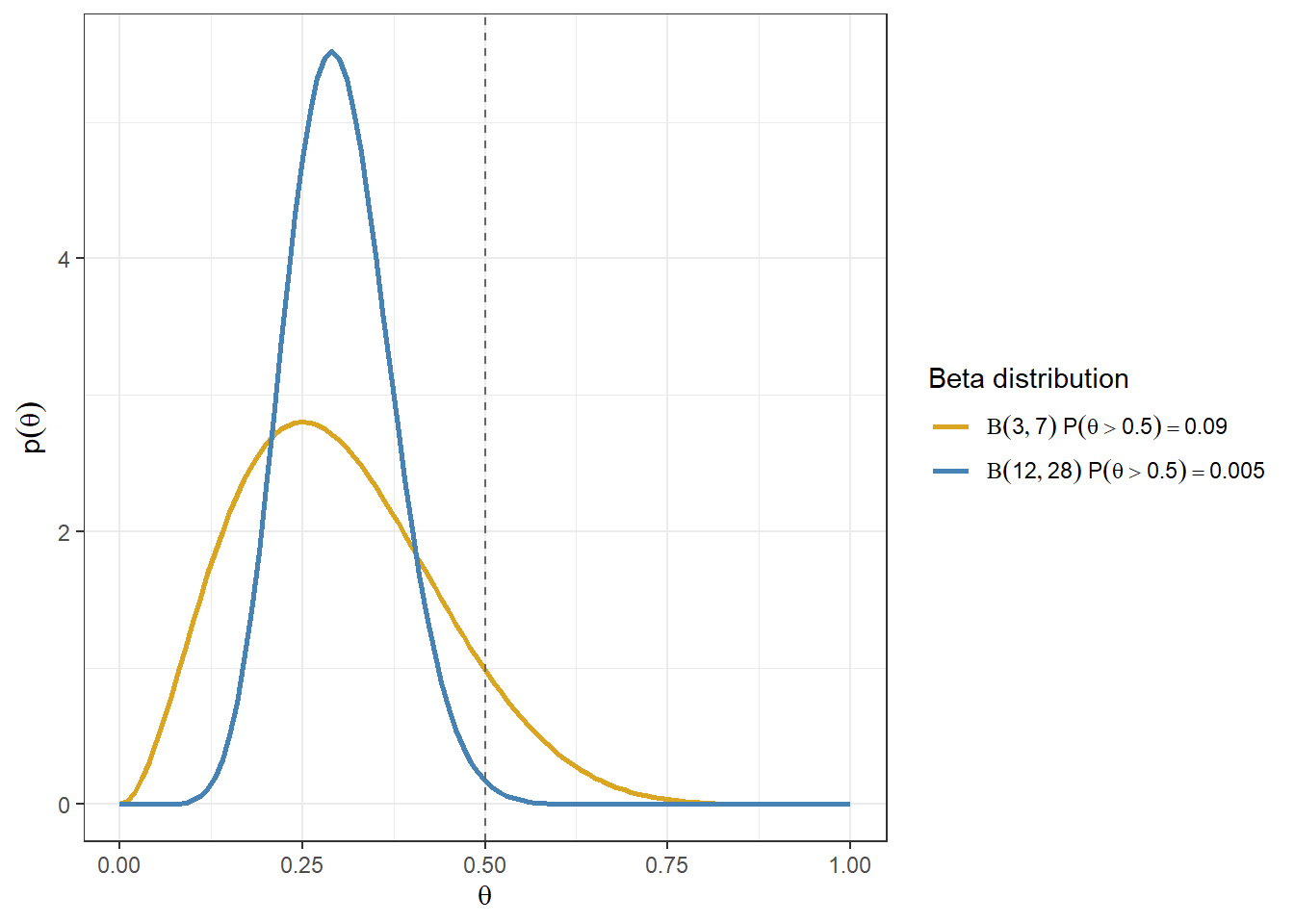
Consider the priors \(Beta(3,7)\) and \(Beta(12,28)\).

• The gold line corresponds to a prior with mean \(3/(3+7)=0.3\).
• The blue line corresponds to a prior with mean \(12/(12+28)=0.3\).

Although these two priors have the same mean, they have different spreads. The prior with larger \(\alpha+\beta\) is more concentrated, so it reflects stronger prior information.

For example, the amount of prior mass above a cutoff such as 0.5 can differ even when the two priors have the same mean.

d <- tibble(theta = seq(from = 0, to = 1, length.out = 101)) %>% 
  expand(theta, a = c(3, 12), b = c(7,28)) %>% 
  mutate(PriorSet = paste0("Beta(",format(a), "," , format(b),")")) %>%
  mutate(priorDensity = dbeta(theta, shape1 = a,shape2 = b))%>%
  filter(a/(a+b)==0.3)
  

# Compute P(theta > 0.5) for each prior
prob_table <- d %>%
  distinct(a, b, PriorSet) %>%
  mutate(prob_gt_05 = pbeta(0.5, shape1 = a, shape2 = b, lower.tail = FALSE),
         label = paste0(PriorSet, "~P(theta>0.5)==", round(prob_gt_05, 3)))

# Merge labels back for plotting
d <- d %>% left_join(prob_table %>% select(PriorSet, label), by = "PriorSet")

ggplot(d, aes(theta, priorDensity, colour = label)) +
  geom_line(size = 1) +
  geom_vline(xintercept = 0.5, linetype = "dashed", colour = "grey40") +
  xlab(expression(theta)) +
  ylab(expression(p(theta))) +
  theme(legend.position = "bottom") +
  scale_colour_manual(values = c("goldenrod", "steelblue"),
                      labels = scales::label_parse(),
                      name = "Beta distribution") +
  theme_bw()

Summarizing the posterior distribution

• Because we know the posterior distribution in closed form, we can easily calculate quantities such as:

  1. the posterior mean: \[E(\theta \mid x) = \frac{\alpha+x}{\alpha+\beta+n}\]
  2. 95% credible intervals
  3. posterior probabilities such as \(P(\theta < 0.2)\), \(P(\theta > 0.5)\), or \(P(0.4 < \theta < 0.6)\)

• These can be used to make direct probability statements about \(\theta\) under the assumed model and prior. For example, we may say that the posterior probability that the adverse event rate is below 0.2 is 0.95.

• We can also generate informative plots to compare priors and posteriors. All of this can be done easily in R.

Interpreting posterior probability

Useful interpretations of posterior probabilities in Bayesian clinical analyses. These thresholds are context-dependent and should be pre-specified when used for decision-making.

Posterior Probability	Verbal Interpretation	Common Usage in Bayesian Clinical Analysis
< 0.05	Very unlikely	Strong evidence against the event or effect
0.05 - 0.20	Unlikely	Little support for the hypothesis
0.20 - 0.40	Somewhat unlikely	Weak evidence; insufficient for a positive conclusion
0.40 - 0.60	Uncertain / Equipoise	Little evidence in either direction
0.60 - 0.80	Somewhat likely	Modest evidence in favour
0.80 - 0.90	Likely	Reasonable evidence; often used in early-phase decisions
0.90 - 0.95	Very likely	Strong evidence
0.95 - 0.99	Highly probable	Very strong evidence
> 0.99	Virtually certain	Near-conclusive evidence

Data overwhelming the prior

• In the beta-binomial model, after observing \(x\) events in \(n\) trials, the posterior is

\[ \theta \mid x \sim Beta(\alpha + x, \beta + n - x), \]

with posterior mean

\[E(\theta \mid x) = \frac{\alpha + x}{\alpha + \beta + n}.\]

• If the sample size is much larger than the prior information, that is, \(n \gg \alpha+\beta\), then the data dominate the posterior.

• For example, with a very weak prior such as \(Beta(0.001,0.001)\),

\[ E(\theta \mid x) = \frac{\alpha + x}{\alpha + \beta + n} \approx \frac{x}{n}. \]

• In that case, the prior has little influence on the posterior mean.

Posterior mean as a weighted average

• The posterior mean can be written as

\[\begin{aligned} E(\theta \mid x) & = \frac{\alpha + x}{\alpha + \beta + n} \\ & = \Big( \frac{\alpha+\beta}{\alpha+\beta+n} \Big)\Big( \frac{\alpha}{\alpha+\beta} \Big) + \Big( \frac{n}{\alpha+\beta+n} \Big)\Big( \frac{x}{n} \Big) \\ & = w \times (\text{prior mean}) + (1-w)\times (\text{sample proportion}), \end{aligned}\]

where

\[ w = \frac{\alpha+\beta}{\alpha+\beta+n}. \]

• So the posterior mean is a weighted average of the prior mean and the observed sample proportion.

• The weight \(w\) depends on the relative amount of prior information compared with the sample size.

• As the sample size increases, the influence of the prior decreases.

3. The Normal-normal model

Parameters with normal priors and normal sampling models

• We continue with a single-parameter model.

• Suppose the data arise from a normal model with known variance \(\sigma^2\):

\[ y \mid \theta \sim N(\theta, \sigma^2). \]

• Here, \(\theta\) is the unknown mean parameter and \(y\) is the observed data.

• Suppose the prior for \(\theta\) is also normal:

\[ \theta \sim N(\mu_0, V_0). \]

• We want to determine the posterior distribution of \(\theta\) given the observed data \(y\).

Normal-normal model

1. The normal model for one data point

• Consider a single observation \(y\) from a normal distribution with mean \(\theta\) and known variance \(\sigma^2\).

• The sampling density of \(y\) given \(\theta\) is

\[ P(y\mid \theta) = \frac{1}{\sqrt{2\pi\sigma^2}} \exp\left\{-\frac{(y-\theta)^2}{2\sigma^2}\right\}, \qquad y \in (-\infty,\infty).\]

• Under this model,
  • \(E(y\mid \theta)=\theta\)
  • \(Var(y\mid \theta)=\sigma^2\)
  • \(SD(y\mid \theta)=\sigma\)
• Since \(y \mid \theta \sim N(\theta,\sigma^2)\), we have

\[ \frac{y-\theta}{\sigma} \sim N(0,1). \]

• Therefore, for a fixed value of \(\theta\), about 95% of observations from this model fall within

\[ \theta \pm 1.96\sigma. \]

This is a statement about the distribution of the data, not a confidence interval for \(\theta\).

2. Prior

We often use a normal prior for \(\theta\):

\[ \theta \sim N(\mu_0, V_0). \]

• \(\mu_0\) is the prior mean.

• \(V_0\) is the prior variance and reflects our uncertainty about \(\theta\).

• It is sometimes convenient to work with precision, defined as the reciprocal of variance:

\[ \tau_0 = \frac{1}{V_0}. \]

• High precision means low variance, so the prior is more concentrated around its mean.

3. Posterior

• With a normal prior and a normal sampling model, the posterior is also normal.

• Using precision notation, write

\[ \theta \sim N(\mu_0, V_0), \qquad y \mid \theta \sim N(\theta,\sigma^2), \]

with

\[ \tau_0 = \frac{1}{V_0}, \qquad \tau_y = \frac{1}{\sigma^2}. \]

• Then the posterior distribution is

\[ \theta \mid y \sim N(\mu_1, V_1), \]

where

\[ \mu_1 = \frac{\tau_0\mu_0 + \tau_y y}{\tau_0+\tau_y}, \qquad V_1 = \frac{1}{\tau_0+\tau_y}. \]

• Equivalently, the posterior precision is

\[ \tau_1 = \tau_0+\tau_y. \]

• So the prior and posterior are both normal distributions.

Posterior mean as a weighted average of the prior mean and the observed value

• Using precision notation,

\[ \tau_y = \frac{1}{\sigma^2_y} \qquad \text{and} \qquad \tau_0 = \frac{1}{V_0}. \]

• The posterior distribution is

\[\theta \mid y \sim N(\mu_1, V_1),\]

where

\[\begin{aligned} \mu_1 &= \Big(\frac{\tau_0}{\tau_0 + \tau_y}\Big)\mu_0 + \Big(\frac{\tau_y}{\tau_0 + \tau_y}\Big)y, \\ V_1 &= \frac{1}{\tau_0 + \tau_y}. \end{aligned}\]

• The posterior mean is therefore a weighted average of the prior mean and the observed value.

• The weights depend on the relative precisions of the prior and the data:

\[\mu_1 = w_0\mu_0 + w_y y,\]

where

\[w_0 = \frac{\tau_0}{\tau_0+\tau_y}, \qquad w_y = \frac{\tau_y}{\tau_0+\tau_y} = 1-w_0.\]

Data overwhelming the prior, and vice versa

• If the prior precision is small relative to the data precision, that is, \(\tau_0 \ll \tau_y\), then

\[ \mu_1 \approx y. \]

In this case, the data dominate the posterior.

• If the data precision is small relative to the prior precision, that is, \(\tau_y \ll \tau_0\), then

\[ \mu_1 \approx \mu_0. \]

In this case, the prior has stronger influence on the posterior.

• In most applications, the posterior mean represents a compromise between prior information and the observed data.

Normal model with multiple observations

• Now consider \(n\) independent observations \(y_1,\ldots,y_n\) from a normal distribution with common mean \(\theta\) and known variance \(\sigma^2\):

\[ y_i \mid \theta \sim N(\theta,\sigma^2), \qquad i=1,\ldots,n. \]

• The joint likelihood is

\[\begin{aligned} P(y_1,\ldots,y_n\mid \theta) &= \prod_{i=1}^n P(y_i\mid \theta) \\ &= \prod_{i=1}^n \frac{1}{\sqrt{2\pi\sigma^2}} \exp\left\{-\frac{(y_i-\theta)^2}{2\sigma^2}\right\}. \end{aligned}\]

• If the prior is \(\theta \sim N(\mu_0,V_0)\), then the posterior is also normal:

\[ \theta \mid y_1,\ldots,y_n \sim N(\mu_n,V_n). \]

• Using precision notation, the posterior mean is

\[\mu_n = \frac{\tau_0\mu_0 + n\tau_y\bar{y}}{\tau_0+n\tau_y} = \Big( \frac{\tau_0}{\tau_0+n\tau_y} \Big)\mu_0 + \Big( \frac{n\tau_y}{\tau_0+n\tau_y} \Big)\bar{y},\]

and the posterior variance is

\[ V_n = \frac{1}{\tau_0+n\tau_y}. \]

• Equivalently, the posterior precision is

\[ \tau_n = \tau_0+n\tau_y. \]

• Here,

\[ \bar{y} = \frac{1}{n}\sum_{i=1}^n y_i, \qquad \tau_y = \frac{1}{\sigma^2}. \]

• Again, the posterior mean is a weighted average of the prior mean and the sample mean.

• As the sample size increases, the weight on the prior decreases and the data increasingly dominate the posterior.

Use of the normal-normal model in clinical applications

• In many clinical applications, we are interested in a parameter such as a mean difference, log-hazard ratio, log-odds ratio, or log-relative risk.

• Suppose we have an estimate of the parameter, and call that estimate \(y\). Let \(\hat{\sigma}_y^2\) be its estimated variance.

• We can treat this estimate as a single summary datum whose sampling distribution depends on the true parameter \(\theta\).

• In large samples, it is often reasonable to use the approximation

\[ y \mid \theta \sim N(\theta,\sigma_y^2), \]

where \(\theta\) is the true parameter value and \(\sigma_y^2\) is the sampling variance of the estimator.

• In practice, we usually replace \(\sigma_y\) by the reported standard error \(\hat{\sigma}_y\).

• If a 95% confidence interval is reported as

\[ y \pm 1.96\hat{\sigma}_y, \]

then we can recover the standard error from the width of the interval.

• This gives us a normal likelihood for \(\theta\) based on the published estimate and its standard error.

Working example - Treatment effect estimate on the mean

• In this example, we simulate data for a small randomized study with \(n=100\) subjects, where 50% are assigned to control and 50% to treatment.

• We then fit a linear regression model to estimate the treatment effect \(\theta\) on the outcome.

n <- 100
set.seed(1234)
treat <- 1*(runif(n, min = 0, max = 1)<0.5)
y <- 5*treat+rnorm(n, mean = 0, sd =10)
fit<-lm(y~treat)
summary(fit)

Call:
lm(formula = y ~ treat)

Residuals:
     Min       1Q   Median       3Q      Max 
-19.8662  -6.7095  -0.5731   5.7503  24.1866 

Coefficients:
            Estimate Std. Error t value Pr(>|t|)  
(Intercept)    1.303      1.423   0.916   0.3618  
treat          4.080      1.918   2.127   0.0359 *
---
Signif. codes:  0 '***' 0.001 '**' 0.01 '*' 0.05 '.' 0.1 ' ' 1

Residual standard error: 9.543 on 98 degrees of freedom
Multiple R-squared:  0.04414,   Adjusted R-squared:  0.03438 
F-statistic: 4.525 on 1 and 98 DF,  p-value: 0.03591

round(confint.default(fit, 'treat', level=0.95),3) # based on asymptotic normality

      2.5 % 97.5 %
treat 0.321   7.84

• Suppose the regression output gives an estimated treatment effect of 4.08 with standard error 1.918.

• We will treat this reported estimate as our observed summary datum \(y\).

• Using the large-sample approximation, we assume

\[ y \mid \theta \sim N(\theta,1.918^2). \]

• Here, 1.918 is the observed standard error of the estimate, and we use it as the standard deviation of the sampling distribution.

• Recall that the standard deviation of the sampling distribution of an estimator is its standard error.

• If the standard error is not reported, but a 95% confidence interval is available, we can recover it from the interval width. For example, if the 95% confidence interval for \(y\) is \((0.321, 7.84)\), then

\[\sigma_y = \frac{7.84-0.321}{2\times 1.96}=1.918.\]

• Suppose we use the prior

\[ \theta \sim N(0, 2\times 1.918^2). \]

• Combining this prior with the likelihood gives the posterior below.

\[\begin{aligned} & \theta \mid y \sim N(\mu_1, V_1) \\ \mu_1 &= \frac{ \frac{1}{prior.sd^2} }{\frac{1}{prior.sd^2} + \frac{1}{se.obs^2} } \times prior.mean + \frac{\frac{1}{se.obs^2}}{\frac{1}{prior.sd^2} + \frac{1}{se.obs^2}} \times y.obs \\ & = \frac{ \frac{1}{2 \times 1.918^2} }{\frac{1}{2 \times 1.918^2} + \frac{1}{1.918^2} } \times 0 + \frac{\frac{1}{1.918^2}}{\frac{1}{2 \times 1.918^2} + \frac{1}{1.918^2}} \times 4.08 = 2.72 \\ V_1 &= \frac{1}{\tau_1}, \\ \tau_1 & = \tau_0 + \tau_y \\ & = \frac{1}{prior.sd^2} + \frac{1}{se.obs^2} \\ & = \frac{1}{2 \times 1.918^2} + \frac{1}{1.918^2} = 0.408. \end{aligned}\]

d <- tibble(theta = seq(from = -10, to = 15, length.out = 200),
         y.obs=4.08,
         se.obs=1.918,
         prior.mean=0,
         prior.sd=sqrt(2)*1.918) %>% 
  mutate(priorDensity = dnorm(theta, prior.mean, prior.sd)) %>%
  mutate(likelihood.0 = dnorm(theta, y.obs, se.obs)) %>%
  mutate(w = (1/se.obs^2)/(1/se.obs^2 + 1/prior.sd^2)) %>%
  mutate(post.prec = 1/se.obs^2 + 1/prior.sd^2) %>%
  mutate(posteriorDensity = dnorm(theta, w*y.obs+(1-w)*prior.mean, sqrt(1/post.prec))) %>%
  mutate(likelihood = likelihood.0/sum(diff(theta)*likelihood.0[-1])) %>%
  pivot_longer(cols=c(priorDensity,likelihood,posteriorDensity),names_to="Function",values_to="p")
  
d$Function <- factor(d$Function, 
                     levels=c("priorDensity","likelihood","posteriorDensity"),
                     labels=c("Prior","Likelihood","Posterior"))

p<-ggplot(d, aes(theta, p,colour=Function))+
  geom_line(size=1)+
  xlab(expression(theta))+
  ylab(expression(p(theta)))+
  theme(legend.position = "bottom")+
  scale_colour_manual(values=c("goldenrod","steelblue","black")) +theme_bw()

p

Working example - Bayesian reanalysis of an RCT: odds ratio

• (Frequentist trial) Effect of a Resuscitation Strategy Targeting Peripheral Perfusion Status vs Serum Lactate Levels on 28-Day Mortality Among Patients With Septic Shock: The ANDROMEDA-SHOCK Randomized Clinical Trial (Hernández et al. 2019)

• (Bayesian reanalysis) Effects of a Resuscitation Strategy Targeting Peripheral Perfusion Status versus Serum Lactate Levels among Patients with Septic Shock: A Bayesian Reanalysis of the ANDROMEDA-SHOCK Trial (Zampieri et al. 2020)

We are interested in making inference about the odds ratio (OR) for 28-day mortality comparing peripheral perfusion-targeted resuscitation with lactate-targeted resuscitation.

This section presents two versions of the Bayesian analysis:

1. a simple teaching example using the crude 2x2 odds ratio from the published counts; and
2. an approximate reconstruction of Zampieri et al.’s neutral prior result using their comparable adjusted frequentist logistic model OR.

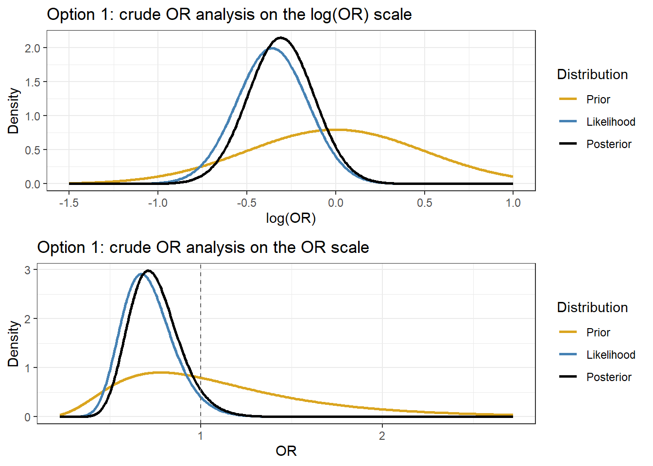
• The first version is useful for illustrating Bayesian updating with a normal likelihood on the log(OR) scale.

• The second version is included to show why the published posterior is more favorable than the crude 2x2 analysis.

Data from the 2x2 table

From the published 28-day mortality counts:

Intervention	Death within 28 days	Alive by 28 days	Total
Peripheral perfusion-targeted resuscitation	74	138	212
Lactate-targeted resuscitation	92	120	212
Total	166	258	424

The crude odds ratio is

\[ \widehat{OR} = \frac{74/138}{92/120} = 0.699. \]

Its large-sample standard error on the log scale is

\[ SE\{\log(\widehat{OR})\} = \sqrt{\frac{1}{74}+\frac{1}{138}+\frac{1}{92}+\frac{1}{120}} \approx 0.200. \]

So the usual Wald 95% confidence interval is

\[ \exp\left[\log(\widehat{OR}) \pm 1.96\times SE\{\log(\widehat{OR})\}\right] = (0.473,\ 1.035). \]

First, Simple Bayesian update using the crude OR

Step 1: Likelihood on the log(OR) scale

Let

\[ \theta = \log(OR). \]

Using the large-sample approximation, we model the observed log odds ratio as

\[ y \mid \theta \sim N(\theta,\sigma_y^2), \]

where

\[ y = \log(0.699) = -0.358, \qquad \sigma_y = 0.200. \]

So the likelihood is

\[ y \mid \theta \sim N(\theta, 0.2^2), \qquad y=-0.358. \]

Step 2: Neutral prior from Zampieri et al.

Zampieri et al. considered a neutral prior with mean 0 and standard deviation 0.5 on the log(OR) scale. We use the same prior here:

\[ \theta \sim N(0,0.5^2). \]

This prior is centered at no effect because \(log(1)=0\). On the OR scale, it corresponds to a prior centered at \(OR=1\), while still allowing both benefit and harm.

Step 3: Posterior under the normal-normal model

Because both the prior and the likelihood are normal on the log(OR) scale, the posterior is also normal:

\[ \theta \mid y \sim N(\mu_1,\sigma_1^2). \]

Using precision notation,

\[ \tau_0 = \frac{1}{0.5^2}=4, \qquad \tau_y = \frac{1}{0.2^2}=25, \qquad \tau_1=\tau_0+\tau_y=29. \]

The posterior mean on the log(OR) scale is

\[ \mu_1 = \frac{\tau_0 \cdot 0 + \tau_y \cdot (-0.358)}{\tau_0+\tau_y} = \frac{4 \times 0 + 25 \times (-0.358)}{29} = -0.309. \]

The posterior variance and standard deviation are

\[ \sigma_1^2 = \frac{1}{29}, \qquad \sigma_1 = \sqrt{\frac{1}{29}} = 0.186. \]

Therefore,

\[ \theta \mid y \sim N(-0.309, 0.186^2). \]

Step 4: Interpreting the posterior on the OR scale

Under this approximation, the posterior distribution of the OR is lognormal.

• The posterior median OR is

\[ \exp(-0.309)=0.734. \]

• The posterior 95% credible interval for the OR is

\[ \exp(-0.309 \pm 1.96\times 0.186) = (0.51,\ 1.06). \]

• We can also calculate posterior probabilities such as \(P(OR<1)\) and \(P(OR<0.8)\).

The published paper used a Bayesian hierarchical logistic regression with covariate adjustment and center random effects.

# simple Bayesian update using the crude 2x2 OR

# crude 2x2 counts
a <- 74   # deaths in peripheral perfusion group
b <- 138  # alive in peripheral perfusion group
c <- 92   # deaths in lactate group
d <- 120  # alive in lactate group

# crude OR and approximate SE on the log scale
or_hat <- (a / b) / (c / d)
y_obs  <- log(or_hat)
se_obs <- sqrt(1/a + 1/b + 1/c + 1/d)

# neutral prior on log(OR)
mu0 <- 0
sd0 <- 0.5
prec0 <- 1 / sd0^2

# posterior on log(OR)
prec_y <- 1 / se_obs^2
prec1  <- prec0 + prec_y
mu1    <- (prec0 * mu0 + prec_y * y_obs) / prec1
sd1    <- 1 / sqrt(prec1)

# display key quantities
cat("Crude OR =", round(or_hat, 3), "\n")

Crude OR = 0.699 

cat("Observed log(OR) =", round(y_obs, 3), "\n")

Observed log(OR) = -0.357 

cat("Observed SE on log scale =", round(se_obs, 3), "\n")

Observed SE on log scale = 0.2 

cat("Posterior mean on log scale =", round(mu1, 3), "\n")

Posterior mean on log scale = -0.308 

cat("Posterior SD on log scale =", round(sd1, 3), "\n")

Posterior SD on log scale = 0.186 

cat("Posterior median OR =", round(exp(mu1), 3), "\n")

Posterior median OR = 0.735 

cat("Posterior 95% CrI for OR = (",
    round(exp(mu1 - 1.96 * sd1), 3), ", ",
    round(exp(mu1 + 1.96 * sd1), 3), ")\n", sep = "")

Posterior 95% CrI for OR = (0.511, 1.057)

# Posterior summaries on the OR scale
res1 <- c(
  posterior_median_OR = exp(mu1),
  lower_95_CrI        = exp(mu1 - 1.96 * sd1),
  upper_95_CrI        = exp(mu1 + 1.96 * sd1),
  `Pr(OR < 1)`        = pnorm(log(1), mean = mu1, sd = sd1),
  `Pr(OR < 0.8)`      = pnorm(log(0.8), mean = mu1, sd = sd1)
)

round(res1, 3)

posterior_median_OR        lower_95_CrI        upper_95_CrI          Pr(OR < 1) 
              0.735               0.511               1.057               0.952 
       Pr(OR < 0.8) 
              0.677 

# Plot on both the log(OR) scale and the OR scale
theta_grid <- seq(-1.5, 1.0, length.out = 400)
or_grid    <- exp(theta_grid)

plot_log <- data.frame(
  x = rep(theta_grid, 3),
  density = c(
    dnorm(theta_grid, mean = mu0,  sd = sd0),
    dnorm(theta_grid, mean = y_obs, sd = se_obs),
    dnorm(theta_grid, mean = mu1,  sd = sd1)
  ),
  Distribution = factor(
    rep(c("Prior", "Likelihood", "Posterior"), each = length(theta_grid)),
    levels = c("Prior", "Likelihood", "Posterior")
  )
)

p1 <- ggplot(plot_log, aes(x, density, colour = Distribution)) +
  geom_line(linewidth = 1) +
  xlab("log(OR)") +
  ylab("Density") +
  theme_bw() +
  scale_colour_manual(values = c("goldenrod", "steelblue", "black")) +
  ggtitle("Option 1: crude OR analysis on the log(OR) scale")

plot_or <- data.frame(
  x = rep(or_grid, 3),
  density = c(
    dnorm(log(or_grid), mean = mu0,  sd = sd0) / or_grid,
    dnorm(log(or_grid), mean = y_obs, sd = se_obs) / or_grid,
    dnorm(log(or_grid), mean = mu1,  sd = sd1) / or_grid
  ),
  Distribution = factor(
    rep(c("Prior", "Likelihood", "Posterior"), each = length(or_grid)),
    levels = c("Prior", "Likelihood", "Posterior")
  )
)

p2 <- ggplot(plot_or, aes(x, density, colour = Distribution)) +
  geom_line(linewidth = 1) +
  geom_vline(xintercept = 1, linetype = "dashed", colour = "grey40") +
  xlab("OR") +
  ylab("Density") +
  theme_bw() +
  scale_colour_manual(values = c("goldenrod", "steelblue", "black")) +
  ggtitle("Option 1: crude OR analysis on the OR scale")

ggarrange(p1, p2, nrow = 2)

Second, approximate reconstruction of the published neutral prior result

Zampieri et al. did not use the crude OR above as their main Bayesian likelihood. Instead, they fit a Bayesian hierarchical logistic regression for 28-day mortality with adjustment for important baseline covariates and a random intercept for center.

To make a simpler approximation that is closer to their published result, we can use:

• the same neutral prior, \[\theta \sim N(0,0.5^2),\]
• but replace the crude OR with the comparable adjusted frequentist logistic-model OR reported in the paper.

For 28-day mortality, Zampieri et al. reported a comparable adjusted frequentist logistic-model result of

\[ OR = 0.61 \quad (95\%\, CI:\ 0.38,\ 0.92). \]

We now use this adjusted OR and CI to define an approximate normal likelihood on the \(log(OR)\) scale.

This second analysis is included to mimic the published neutral prior posterior more closely. It still does not reproduce the paper exactly, because:

• we do not have the full patient-level data in this worked example,
• we are not fitting the hierarchical logistic regression directly,
• and we are replacing the full regression likelihood by a normal approximation based on the published adjusted OR and CI.

# Approximate reconstruction of Zampieri's neutral-prior result
# using the published comparable adjusted logistic-model OR

# published comparable adjusted frequentist logistic-model result
or_adj  <- 0.61
ci_low  <- 0.38
ci_high <- 0.92

# approximate likelihood on log(OR) scale
y_obs2  <- log(or_adj)
se_obs2 <- (log(ci_high) - log(ci_low)) / (2 * 1.96)

# same neutral prior
mu0_2 <- 0
sd0_2 <- 0.5
prec0_2 <- 1 / sd0_2^2

# posterior
prec_y2 <- 1 / se_obs2^2
prec2   <- prec0_2 + prec_y2
mu2     <- (prec0_2 * mu0_2 + prec_y2 * y_obs2) / prec2
sd2     <- 1 / sqrt(prec2)

cat("Adjusted OR used for approximation =", round(or_adj, 3), "\n")

Adjusted OR used for approximation = 0.61 

cat("Approximate SE on log scale =", round(se_obs2, 3), "\n")

Approximate SE on log scale = 0.226 

cat("Approximate posterior median OR =", round(exp(mu2), 3), "\n")

Approximate posterior median OR = 0.663 

cat("Approximate posterior 95% CrI for OR = (",
    round(exp(mu2 - 1.96 * sd2), 3), ", ",
    round(exp(mu2 + 1.96 * sd2), 3), ")\n", sep = "")

Approximate posterior 95% CrI for OR = (0.443, 0.992)

# Posterior summaries for the approximate reconstruction
res2 <- c(
  posterior_median_OR = exp(mu2),
  lower_95_CrI        = exp(mu2 - 1.96 * sd2),
  upper_95_CrI        = exp(mu2 + 1.96 * sd2),
  `Pr(OR < 1)`        = pnorm(log(1), mean = mu2, sd = sd2),
  `Pr(OR < 0.8)`      = pnorm(log(0.8), mean = mu2, sd = sd2)
)

round(res2, 3)

posterior_median_OR        lower_95_CrI        upper_95_CrI          Pr(OR < 1) 
              0.663               0.443               0.992               0.977 
       Pr(OR < 0.8) 
              0.819 

Under the neutral prior, Zampieri et al. reported a posterior OR of approximately 0.65 (0.43, 0.96).

Summary of Conjugate priors & models

• There are a small number of prior-likelihood pairs where the prior and the posterior are in the same family (e.g., both beta, both normal): these are called conjugate models

• These posterior distributions can be computed without specialized software

• These examples are useful for illustrating how Bayesian methods combine prior information with data

• They have only limited practical usefulness - limits on types priors, limits on number of parameters

• They are useful teaching tools, soon we will see how we can extend beyond these simple models

4. Bayesian vs Frequentist: A Tale of Two Designs

To make the comparison concrete, consider a simple two-arm randomized controlled trial comparing treatment versus control on a continuous outcome.

We assume:

• The treatment effect of interest is \[\delta = \mu_T - \mu_C,\] the difference in mean outcome between the treatment and control groups.
• The minimally clinically important difference (MCID) is \(\delta = 1\). This means a difference of 1 unit is the smallest effect that would be considered clinically meaningful.
• The outcome standard deviation is assumed known and equal to \(\sigma = 2\) (variance \(=4\)).
• Outcomes are normally distributed.

We will design the same trial in two different ways:

• a frequentist design, based on controlling long-run error rates, and
• a Bayesian design, based on posterior probabilities and a pre-specified decision rule.

The main questions are the same in both cases:

• How many patients do we need?
• What rule will we use to declare success?
• How often will that rule lead to a correct or incorrect conclusion?

4.1 Frequentist Design

In a frequentist design, we choose the sample size so that the final analysis has acceptable long-run operating characteristics.

Here we specify:

• Type I error: \(\alpha = 0.05\) (two-sided)

  This means that if there is truly no treatment effect, the trial will incorrectly declare a difference about 5% of the time in the long run.

• Power: \(1-\beta = 0.80\)

  This means that if the true treatment effect is the MCID, the trial has an 80% chance of detecting it.

For a two-sample \(z\)-test with equal allocation, the required sample size per arm is

\[n = \frac{2\sigma^2(z_{1-\alpha/2} + z_{1-\beta})^2}{\delta^2}\]

where \(z_{1-\alpha/2}=1.96\) and \(z_{1-\beta}=0.842\).

# Frequentist sample size
delta <- 1       # MCID
sigma <- 2       # SD
alpha <- 0.05    # Type I error
power <- 0.80    # Power

z_alpha <- qnorm(1 - alpha/2)
z_beta  <- qnorm(power)

n_per_arm <- ceiling(2 * sigma^2 * (z_alpha + z_beta)^2 / delta^2)
n_total   <- 2 * n_per_arm

cat("Required n per arm:", n_per_arm, "\n")

Required n per arm: 63 

cat("Required total n:  ", n_total, "\n")

Required total n:   126 

What the frequentist design gives you:

• A fixed sample size chosen before the trial starts
• A decision rule: reject \(H_0: \delta = 0\) if \(p < 0.05\)
• A long-run guarantee on error rates: under repeated use of this design, the false positive rate is controlled at 5%

What it cannot give you: - A probability statement such as \(P(\delta > 1 \mid \text{data})\), the probability the treatment is clinically meaningful given what you observed.

4.2 Bayesian Trial Design

A Bayesian trial design answers the same practical questions as a frequentist design, but it does so in a different way.

We still need to decide:

1. How to model the data
2. What prior information to use
3. What rule will count as a successful trial
4. How often that rule leads to the right or wrong conclusion

The main difference is that a Bayesian design is built around the posterior distribution of the treatment effect after seeing the data.

Sampling Model

Assume \[Y_{ij} \mid \mu_j \sim N(\mu_j, \sigma^2), \qquad j \in \{T, C\}\]

where:

• \(j=T\) denotes the treatment arm
• \(j=C\) denotes the control arm
• \(\mu_T\) and \(\mu_C\) are the group means
• \(\sigma^2\) is the common outcome variance

Define the treatment effect as

\[\Delta = \mu_T - \mu_C.\]

If each arm has sample size \(n\), then the observed difference in sample means

\[d = \bar{Y}_T - \bar{Y}_C\]

has sampling distribution

\[\bar{Y}_T - \bar{Y}_C \mid \Delta \sim N\left(\Delta,\; \frac{2\sigma^2}{n}\right) = N\left(\Delta,\; \frac{8}{n}\right).\]

So in this setting, the data can be summarized by the observed mean difference \(d\), and the uncertainty around \(d\) decreases as the sample size increases.

Prior

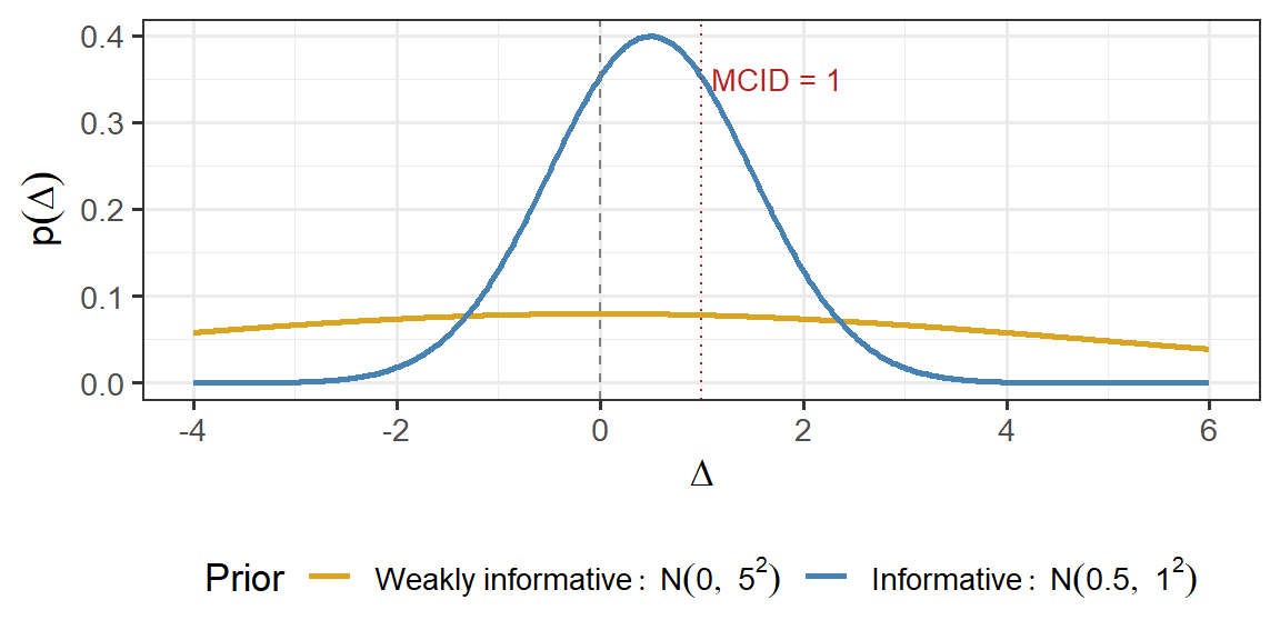
We consider two prior distributions for \(\Delta\).

Weakly informative prior
This prior reflects little prior knowledge about the treatment effect: \[\Delta \sim N(0, 5^2)\]

• It is centred at 0, so it does not assume benefit or harm in advance
• Its 95% prior interval is approximately \((-9.8,\ 9.8)\), which is very wide relative to the MCID
• In practice, this prior contributes very little information

Informative prior
This prior reflects earlier evidence, such as a pilot study or phase II trial, suggesting a modest positive effect: \[\Delta \sim N(0.5, 1^2)\]

• It is centred at 0.5, suggesting a positive effect on average
• Its 95% prior interval is approximately \((-1.5,\ 2.5)\), so it still allows no effect and harmful effects
• Compared with the weak prior, it contributes more information and can reduce the amount of trial data needed to reach a conclusion

priors <- list(
  "Weakly~informative:~N(0,~5^2)"  = c(mean = 0,   sd = 5),
  "Informative:~N(0.5,~1^2)"       = c(mean = 0.5, sd = 1)
)

tibble(
  Delta = seq(-4, 6, length.out = 500)
) %>%
  expand_grid(prior_name = names(priors)) %>%
  mutate(
    prior_mean    = map_dbl(prior_name, ~ priors[[.x]]["mean"]),
    prior_sd      = map_dbl(prior_name, ~ priors[[.x]]["sd"]),
    density       = dnorm(Delta, mean = prior_mean, sd = prior_sd),
    prior_label   = factor(prior_name, levels = names(priors))
  ) %>%
  ggplot(aes(x = Delta, y = density, colour = prior_label)) +
  geom_line(linewidth = 1) +
  geom_vline(xintercept = 0,    linetype = "dashed", colour = "grey50") +
  geom_vline(xintercept = 1,    linetype = "dotted", colour = "firebrick") +
  annotate("text", x = 1.1, y = 0.35, label = "MCID = 1", 
           colour = "firebrick", hjust = 0, size = 3.5) +
  scale_colour_manual(
    values = c("goldenrod", "steelblue"),
    labels = scales::label_parse()
  ) +
  labs(x      = expression(Delta),
       y      = expression(p(Delta)),
       colour = "Prior") +
  theme_bw(base_size = 13) +
  theme(legend.position = "bottom")

Figure 1: Prior distributions on Delta. The weakly informative prior expresses minimal prior knowledge. The informative prior reflects a pilot study suggesting modest benefit.

Bayesian Decision Rule

At the end of the trial, we compute the posterior probability that the treatment is better than control.

We declare the trial successful if

\[\Pr(\Delta > 0 \mid \text{data}) > 0.975.\]

In words, we require the posterior probability of benefit to exceed 97.5%.

This is a stringent superiority rule. In settings like this one, it is often viewed as broadly comparable to a conventional frequentist standard, although it is not identical to a two-sided \(p < 0.05\) test.

Power Condition

To determine the sample size, we ask the following question:

If the true treatment effect equals the MCID, how often will this Bayesian decision rule declare success?

So we look for the smallest \(n\) such that, when the true effect is \(\Delta = 1\), the probability of success is at least 0.80:

\[P\Big(P(\Delta > 0 \mid \text{data}) > 0.975 \;\Big|\; \Delta = \text{MCID}\Big) \geq 0.80.\]

This plays the same role as power in a frequentist design: it tells us how likely the trial is to detect a clinically meaningful effect when that effect is truly present.

Normal-Normal Posterior

Because both the prior and the sampling model are normal, the posterior distribution is also normal.

Given the observed mean difference \(d = \bar{Y}_T - \bar{Y}_C\),

\[\Delta \mid \text{data} \sim N(\mu_1, \tau_1^{-1})\]

where

\[\tau_1 = \frac{1}{\sigma_0^2} + \frac{n}{8}, \qquad \mu_1 = \frac{(\mu_0/\sigma_0^2) + (n/8)\,d}{\tau_1}.\]

This formula shows that the posterior mean is a weighted average of:

• the prior mean \(\mu_0\), and
• the observed treatment effect \(d\)

As the sample size increases, the data become more precise and carry more weight in the posterior.

# Parameters
sigma  <- 2    # SD per group
mcid   <- 1    # MCID
gamma  <- 0.975 # posterior probability threshold
n_sim  <- 10000
set.seed(123)

# Two priors to compare
priors <- list(
  "N(0,5^2)"  = c(mean = 0,   sd = 5),
  "N(0.5,1^2)"   = c(mean = 0.5, sd = 1)
)

# Simulate one trial and return P(Delta > 0 | data)
run_bayes_trial <- function(n, true_delta, sigma, prior_mean, prior_sd) {
  
  y_trt  <- rnorm(n, mean = true_delta, sd = sigma)
  y_ctrl <- rnorm(n, mean = 0,          sd = sigma)
  d      <- mean(y_trt) - mean(y_ctrl)
  
  # Normal-Normal posterior
  se2        <- 2 * sigma^2 / n
  prec_prior <- 1 / prior_sd^2
  prec_lik   <- 1 / se2
  prec_post  <- prec_prior + prec_lik
  mu_post    <- (prec_prior * prior_mean + prec_lik * d) / prec_post
  sd_post    <- sqrt(1 / prec_post)
  
  # P(Delta > 0 | data)
  1 - pnorm(0, mean = mu_post, sd = sd_post)
}

Operating Characteristics by Simulation

Even though the decision rule is Bayesian, we can still evaluate its performance using repeated simulation.

In particular, we examine:

• False positive rate: how often the rule declares success when the true effect is \(\Delta = 0\)
• Power: how often the rule declares success when the true effect is \(\Delta = 1\), the MCID

This is an important idea in Bayesian trial design:
we can use Bayesian inference for the final decision, while still checking frequentist-style operating characteristics such as false positive rate and power.

sample_sizes <- seq(60, 70, by = 1)

# Compute OC for each prior
oc_results <- map_dfr(names(priors), function(prior_name) {
  
  pm <- priors[[prior_name]]["mean"]
  ps <- priors[[prior_name]]["sd"]
  
  map_dfr(sample_sizes, function(n) {
    
    null_sims <- replicate(n_sim,
      run_bayes_trial(n, true_delta = 0, sigma = sigma,
                     prior_mean = pm, prior_sd = ps))
    
    alt_sims <- replicate(n_sim,
      run_bayes_trial(n, true_delta = mcid, sigma = sigma,
                     prior_mean = pm, prior_sd = ps))
    
    tibble(
      prior_name     = prior_name,
      n_per_arm      = n,
      false_pos_rate = mean(null_sims > gamma),
      power          = mean(alt_sims  > gamma)
    )
  })
})


# Find minimum n meeting both criteria for each prior
bayes_n <- oc_results %>%
  filter(false_pos_rate <= 0.05, power >= 0.80) %>%
  group_by(prior_name) %>%
  slice_min(n_per_arm) %>%
  ungroup()

bayes_n %>%
  mutate(
    total_n        = 2 * n_per_arm,
    false_pos_rate = round(false_pos_rate, 3),
    power          = round(power, 3)
  ) %>%
  select(prior_name, n_per_arm, total_n, false_pos_rate, power) %>%
  knitr::kable(
    col.names = c("Prior", "n per arm", "Total n",
                  "False Positive Rate", "Power"),
    caption   = "Minimum sample size meeting operating characteristic 
                 targets (false positive rate <= 5%, power >= 80%) 
                 by prior distribution."
  )

Minimum sample size meeting operating characteristic targets (false positive rate <= 5%, power >= 80%) by prior distribution.

Prior	n per arm	Total n	False Positive Rate	Power
N(0,5^2)	63	126	0.024	0.801
N(0.5,1^2)	61	122	0.028	0.804

Operating characteristics of the Bayesian design under two priors. The success rule is P(Delta > 0 | data) > 0.975, evaluated at Delta = 0 (false positive rate) and Delta = 1 (MCID, power). Dashed lines show the targets. Vertical dotted lines mark the minimum n for each prior.

How prior information changes the design

Table 1: Design comparison across frequentist and two Bayesian designs. All designs target 80% power at the MCID with false positive rate controlled at 5%.

	Frequentist	Bayesian (Weak Prior)	Bayesian (Informative Prior)
Sample size (per arm)	63	63	61
Total sample size	126	126	122
Success rule	p < 0.05	P(Delta > 0 | data) > 0.975	P(Delta > 0 | data) > 0.975
Power condition	80% power at Delta = MCID	80% success at Delta = MCID	80% success at Delta = MCID
Prior belief	None	N(0, 25)	N(0.5, 1)

All three designs are being evaluated against the same practical standards:

• they should have at least 80% power when the true effect equals the MCID, and
• they should keep the false positive rate acceptably low

The main lessons are:

• The weakly informative Bayesian design gives a sample size very similar to the frequentist design, because the prior adds little information
• The informative Bayesian design can require fewer patients, because prior evidence contributes information
• In both Bayesian designs, the final result is a posterior distribution for \(\Delta\), not just a binary reject/do not reject decision

Bayesian inference does not automatically solve statistical power problems. Its main advantages are:
i) the ability to incorporate prior information naturally, and
ii) the natural extension to adaptive monitoring and other flexible trial design features.

Connection to FDA 2026 Draft Guidance

The FDA draft guidance on Bayesian methods (January 2026) explicitly endorses exactly this approach: evaluating Bayesian designs via simulated operating characteristics to demonstrate that false positive rates and power meet regulatory expectations. This means Bayesian and frequentist designs can be held to the same accountability standard, while the Bayesian design offers richer inference.

References

Hernández, Glenn, Gustavo A Ospina-Tascón, Lucas Petri Damiani, Elisa Estenssoro, Arnaldo Dubin, Javier Hurtado, Gilberto Friedman, et al. 2019. “Effect of a Resuscitation Strategy Targeting Peripheral Perfusion Status Vs Serum Lactate Levels on 28-Day Mortality Among Patients with Septic Shock: The ANDROMEDA-SHOCK Randomized Clinical Trial.” Jama 321 (7): 654–64.

Zampieri, Fernando G, Lucas P Damiani, Jan Bakker, Gustavo A Ospina-Tascón, Ricardo Castro, Alexandre B Cavalcanti, and Glenn Hernandez. 2020. “Effects of a Resuscitation Strategy Targeting Peripheral Perfusion Status Versus Serum Lactate Levels Among Patients with Septic Shock. A Bayesian Reanalysis of the ANDROMEDA-SHOCK Trial.” American Journal of Respiratory and Critical Care Medicine 201 (4): 423–29.