Bayesian Hierarchical Linear Regression

Learning Objectives

Learn how to fit regression model with correlated data with brms

1. Hierarchical models

Often models have more complex structures than the ones described by likelihood and priors and simple relationships between data and parameters
In these models data and parameters participate in relationships of hierarchical fashion
- e.g., Correlated and clustering data structures, such as measures within patients, patients within clinics etc.
Bayesian models deal with hierarchical models in a natural and intuitive way (Bürkner 2017)
Source of correlation in clustered (or longitudinal) data
- between-individual heterogeneity on i) mean and ii) velocity (rate of change; slop)
- Within-individual/cluster homogeneity

1.1 Bayesian Hierarchical Models

Often Bayesian models can we written in the following layers of the hierarchy
1. Data Layer \(Y \mid \theta\), the likelihood for the observed data \(Y\) given model parameters \(\theta\).
2. Adaptive/Structural Priors \(\theta \mid \alpha, \beta\), the model for parameter \(\theta\) that defined by the latent data generating process governed by the hyperparameters \(\alpha\) and \(\beta\)
3. Hyper Priors \(\alpha\) and \(\beta\) as hyper parameters.

1.1 Clustered data (Multi-level)

Example: Developmental toxicity study of ethylene glycol (EG) (Price et al. 1985)
The data are from a development toxicity study of ethylene glycol (EG).
Ethylene glycol is a high-volume industrial chemical used in many applications.
In a study of laboratory mice conducted through the National Toxicology Program (NTP), EG was administered at doses of 0, 750, 1500, or 3000 mg/kg/day to 94 pregnant mice (dams) over the period of major organogenesis, beginning just after implantation.
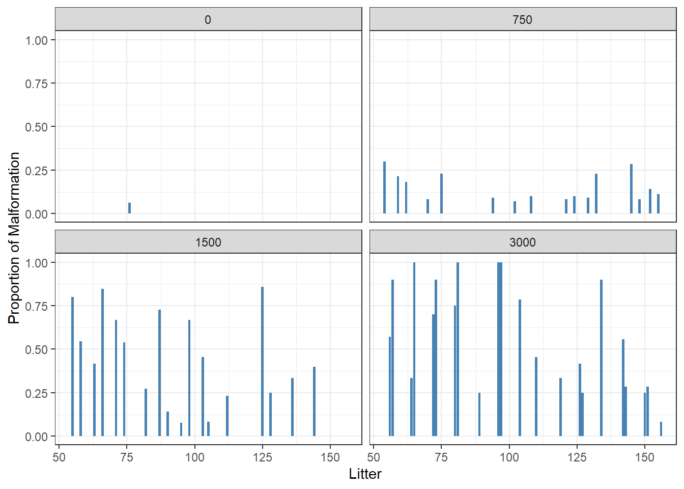
Following sacrifice, fetal weight and evidence of malformations were recorded
Let’s first read in the data
- This data set is in a long format
- we can see each row represents a mouse.
- Mice are nested within the litter. We have a two-level data!

Code

ntp <- read.table("data/ntp-data.txt", header = TRUE)
colnames(ntp) <- c("Litter", "Dose", "Weight", "Malformation")
ntp <- ntp %>%
  group_by(Litter) %>%
  mutate(Litid = row_number()) %>% # seq id for each litter
  mutate(FetalID = paste0(Litter, ".", Litid)) %>% # FetalID = LitID.tempid
  select(-Litid) # remove tempid from toxic2

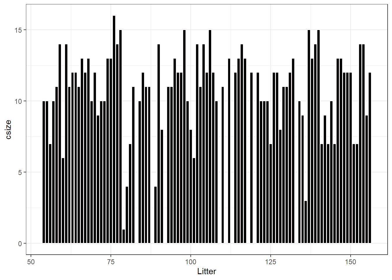
Number of doses in each group and number of fetuses in each litter

Code

cluster <- ntp %>% group_by(Dose) %>%
  summarize(nlitter = n_distinct(Litter), nfetal = n_distinct(FetalID))

cluster %>% datatable(
  rownames = FALSE,
  options = list(
    columnDefs = list(list(className = 'dt-center', 
                      targets = 0:2))))

Code

clustersize <- ntp %>% group_by(Litter) %>% summarise(csize = n_distinct(FetalID))

clustersize %>%
ggplot(aes(x = Litter, y = csize)) +
geom_bar(stat = "identity", fill = "black", color = "snow1")+
  theme_bw()

Visualize relationship between fetal malformation and dose

Code

ntp %>%
  group_by(Dose, Litter) %>%
  summarise(fmalprop = mean(Malformation)) %>%
  ggplot(aes(x = Litter, y = fmalprop)) +
  geom_bar(stat = "identity", fill = "steelblue") +
  ylab("Proportion of Malformation")+
  facet_wrap(~Dose)+
  theme_bw()

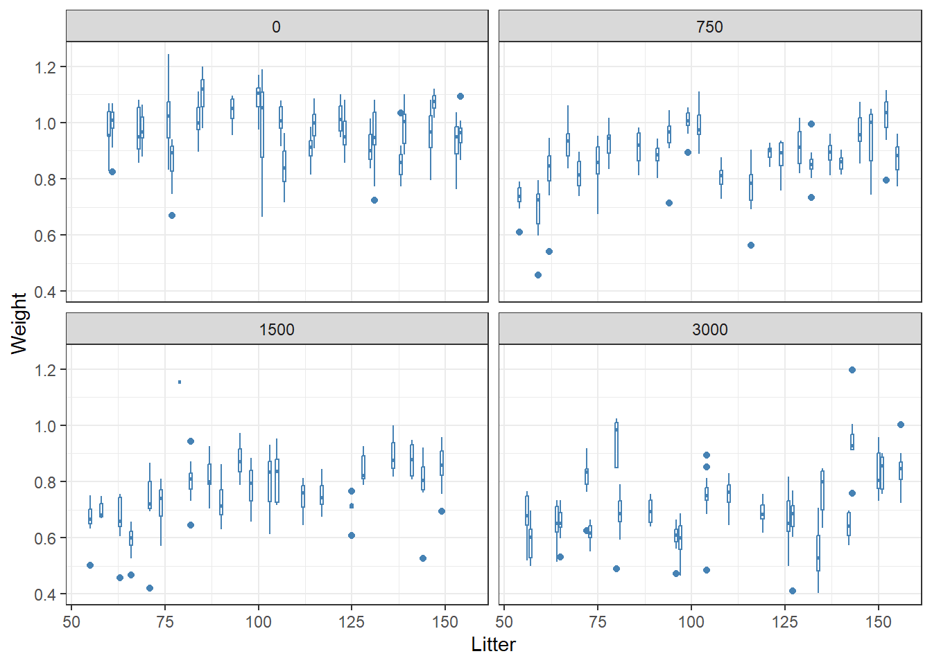
Visualize relationship between fetal weight and dose

Code

ntp %>%
  ggplot(aes(x = Litter, y = Weight)) +
  geom_boxplot(aes(group = Litter), color = "steelblue") +
  facet_wrap(~Dose)+
  theme_bw()

Code

ntp <- ntp %>% 
  mutate(Dose = factor(Dose, levels = c("0","750","1500","3000")))

Suppose we are interested to assess the effect of dose on fetal weight.
The data on fetal weight from this experiment are clustered, with observations on the fetuses nested within litters.

1.3 Normal hierarchical model with random intercept (model 1)

data structure: model of fetal weight within each litter (index by j) \[ Y_{ij} \mid \mu_j, \sigma_y \sim N(\mu_j, \sigma_y^2)\]
adaptive priors on litter-level mean

\[\mu_j \mid \mu, \sigma_\mu \sim N(\mu, \sigma_u^2)\]

hyperparameter priors on \(\mu\), \(\sigma_u\) as well as global prior for \(\sigma_y\)
Variability within litter by dose
- in this model, only \(\beta_{0j}\) depends on litter
- \(\beta_{1}\) is shared across all litter \(j\), the expected change in fetal weight comparing between various dosage to reference level (dose = 0)
- \(\sigma_y\) measures Within-group variability around the mean regression model \(\beta_{0j} + \beta_{1} \ dose_{ij}\)

\[\mu_{ij} = \beta_{0j} + \beta_{1} \ dose_{ij}\]

specifying our hierarchical random intercepts model (update with \(\beta\)):

\[ Y_{ij} \mid \beta_{0j}, \beta_{1}, \sigma_y \sim N(\beta_{0j} + \beta_{1} \ dose_{ij}, \sigma_y^2) \]

\[\beta_{0j} \mid \beta_{0}, \sigma_0^2\]

\[\beta_{0} \sim N(0,10)\] \[\beta_{1} \sim N(0,10)\] \[\sigma_y \sim HalfCauchy(10)\] \[\sigma_0 \sim HalfCauchy(10)\]

Code

fit2 <- brm(data = ntp,
            family= gaussian(),
            Weight ~ Dose + (1|Litter),  
            prior = c(prior(normal(0, 10), class = Intercept),
                      prior(normal(0, 10), class = b),
                      prior(cauchy(0, 10), class = sd),
                      prior(cauchy(0, 10), class = sigma)),
            iter = 10000,
            warmup = 8000,
            chains = 4,
            cores = 4, 
            seed = 123, 
            silent = 2,
            refresh = 0)
# saveRDS(fit2, "data/chp4_h_example2")

Code

fit2 <- readRDS("data/chp4_h_example2")
summary(fit2)

 Family: gaussian 
  Links: mu = identity; sigma = identity 
Formula: Weight ~ Dose + (1 | Litter) 
   Data: ntp (Number of observations: 1027) 
  Draws: 4 chains, each with iter = 10000; warmup = 8000; thin = 1;
         total post-warmup draws = 8000

Group-Level Effects: 
~Litter (Number of levels: 94) 
              Estimate Est.Error l-95% CI u-95% CI Rhat Bulk_ESS Tail_ESS
sd(Intercept)     0.09      0.01     0.07     0.10 1.00     1327     2096

Population-Level Effects: 
          Estimate Est.Error l-95% CI u-95% CI Rhat Bulk_ESS Tail_ESS
Intercept     0.97      0.02     0.94     1.01 1.00      934     1686
Dose750      -0.09      0.03    -0.14    -0.04 1.00     1059     1878
Dose1500     -0.19      0.03    -0.25    -0.14 1.00     1017     1607
Dose3000     -0.26      0.03    -0.31    -0.21 1.00      997     2009

Family Specific Parameters: 
      Estimate Est.Error l-95% CI u-95% CI Rhat Bulk_ESS Tail_ESS
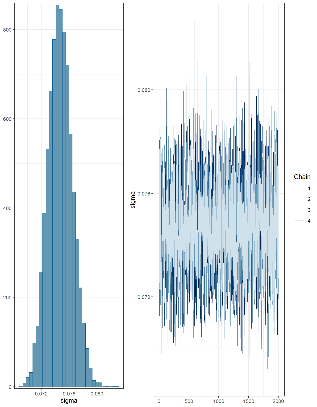
sigma     0.07      0.00     0.07     0.08 1.00     7140     5025

Draws were sampled using sampling(NUTS). For each parameter, Bulk_ESS
and Tail_ESS are effective sample size measures, and Rhat is the potential
scale reduction factor on split chains (at convergence, Rhat = 1).

Code

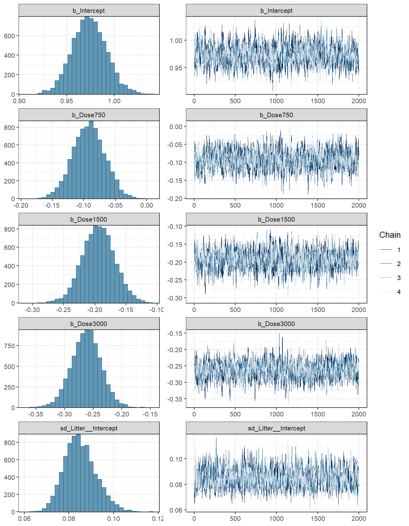
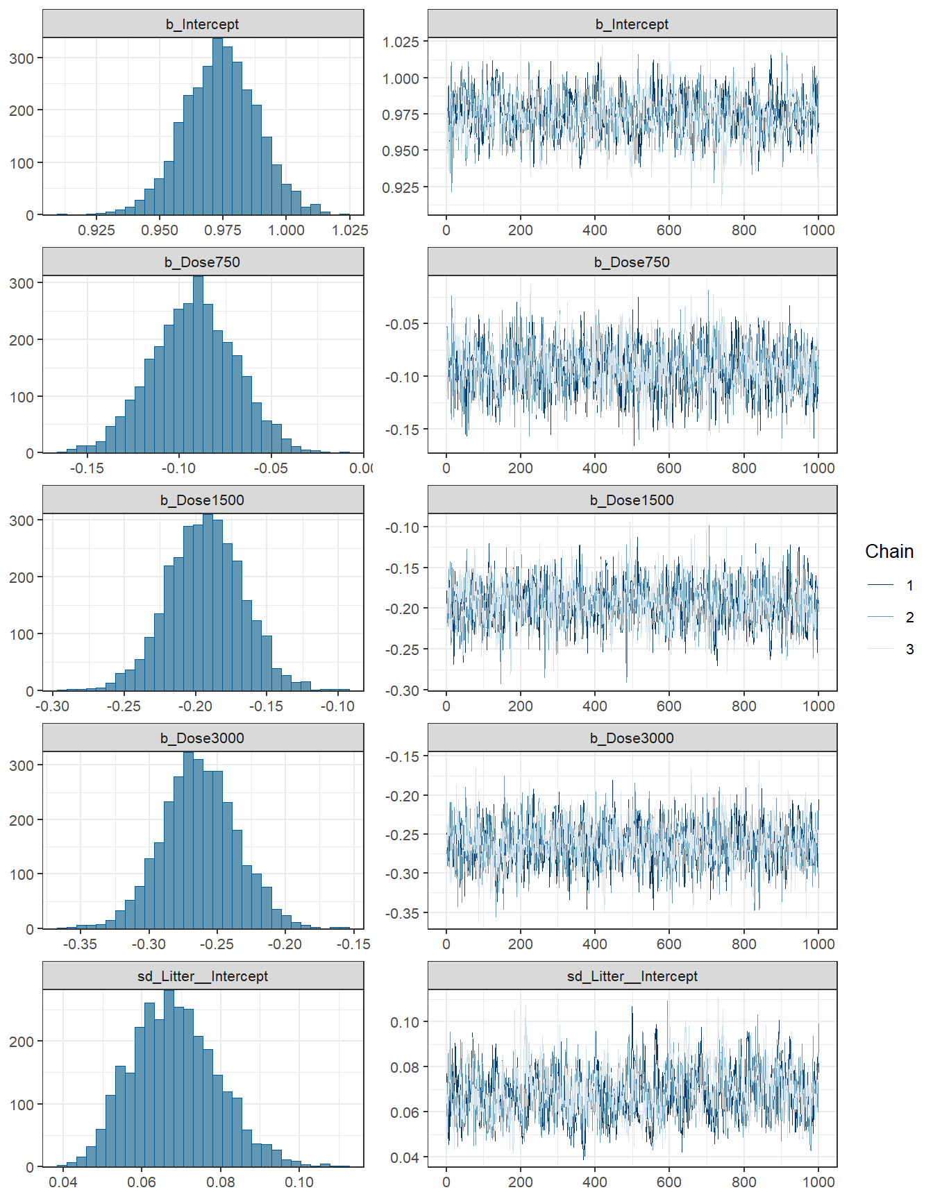
# checking traceplot
fit2 %>% plot(combo = c("hist", "trace"), widths = c(1, 1.5),
      theme = theme_bw(base_size = 10))

`stat_bin()` using `bins = 30`. Pick better value with `binwidth`.
`stat_bin()` using `bins = 30`. Pick better value with `binwidth`.

Code

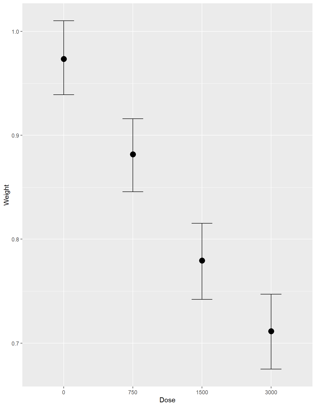
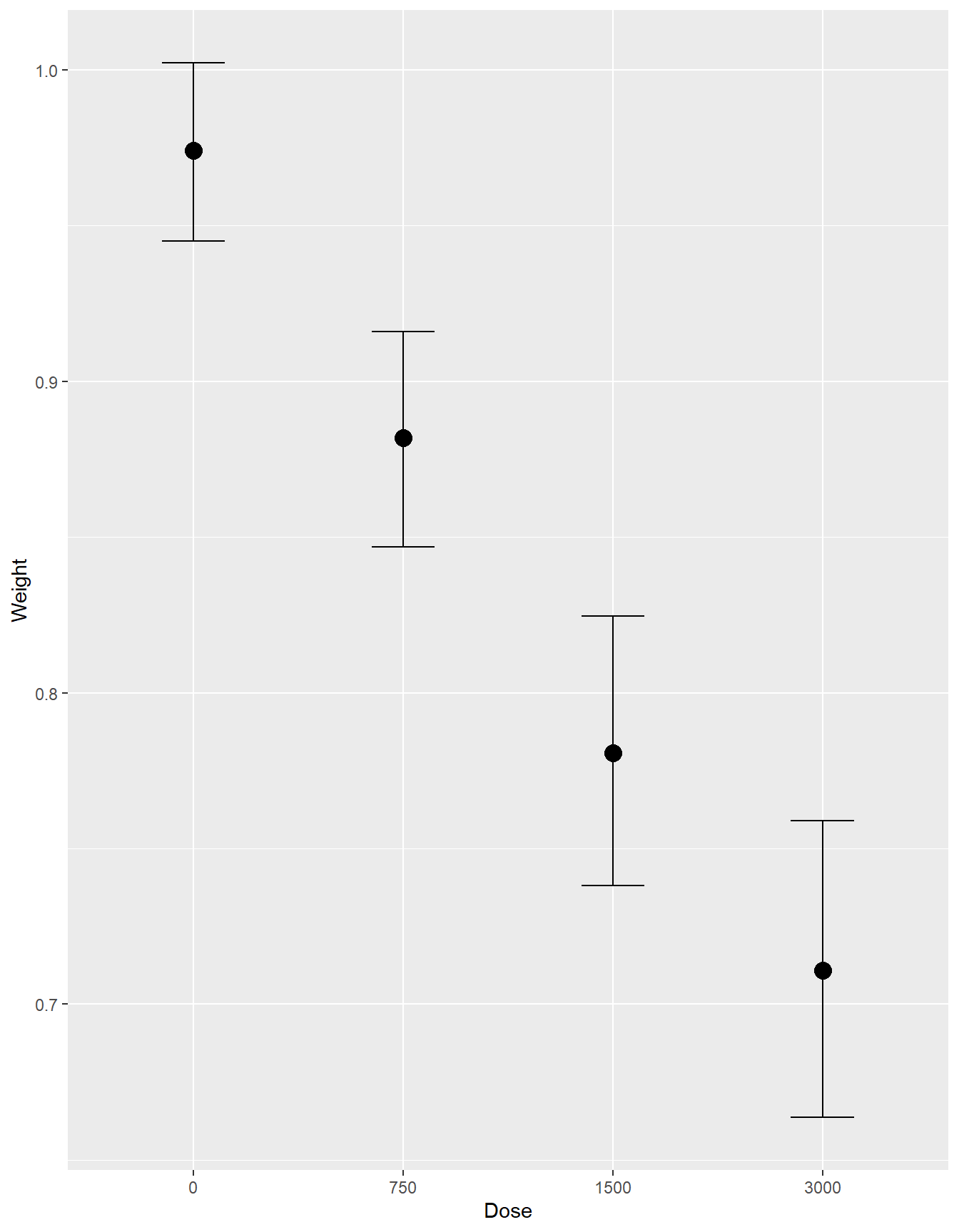
conditional_effects(fit2)

Interpretation
Fixed effects

Term	Posterior mean	95% Credible Interval	Interpretation (baseline at dose 0)
Intercept	0.97	0.94 - 1.01	Expected Weight when Dose = 0, averaged over all litters.
Dose 750	-0.09	-0.14 - -0.04	Avg. change (decrease) when moving from 0 to 750
Dose 1500	-0.19	-0.25 - -0.14	Avg. change at 1500
Dose 3000	-0.26	-0.31 - -0.21	Largest average decrease at 3000

All dose coefficients are negative and their intervals exclude 0 indicating strong evidence that higher doses lower weight.

Random effect (between-litter variability)

Parameter	Posterior SD	95 % Credible Interval	Meaning
sd(Intercept)	0.09	0.07 - 0.10	Litters differ in baseline weight by roughly \(\pm\) 0.09 around the grand mean.

Only baseline (intercept) varies; slope variation was not included in this model.

Within-litter (residual) variance, \(\sigma = 0.07 (0.07 - 0.08)\), after accounting for dose and litter baseline, individual vary by about 0.07 units.
The adjusted ICC represents the proportion of variance of the outcome that are due to between-level (e.g., between-group, between-person) differences
- Does not consider fixed effect! In this case, adjusted ICC does not feature variation caused by dose.

\[\rho_{adj} = \frac{\sigma_0^2}{\sigma_0^2 + \sigma^2}\]

where \(\sigma_0^2\) is the between-level SD, which is the SD of cluster means (i.e., variability between litters) and \(\sigma\) is the observation-specific SD (i.e., variability within a litter)
The conditional ICC considers variation with fixed effect, in this case dose.

\[\rho_{c} = \frac{\sigma_0^2}{\sigma_0^2 + \sigma^2 + \sigma_f^2}\]

\[\sigma_f^2 = var(\sum_{m=1}^p \beta_m x_{mij})\]

reference: (Nakagawa, Johnson, and Schielzeth 2017) doi: 10.1098/rsif.2017.0213
We can use the posterior draws of the two SD to compute the posterior for the adjusted ICC:

Code

# Computing ICC
# 1. Obtain posterior draws of tau and sigma
sd_m2 <- VarCorr(fit2, summary = FALSE)
draws_tau <- sd_m2$Litter$sd[ , "Intercept"]  # tau
draws_sigma <- sd_m2$residual__$sd[ , 1]  #sigma
# 2. Compute draws for adjusted ICC
draws_icc <- draws_tau^2 / (draws_tau^2 + draws_sigma^2)
# quantile of posterior adjusted ICC
quantile(draws_icc, p=c(0.5, 0.025,0.975))

      50%      2.5%     97.5% 
0.5621332 0.4775515 0.6454052

Code

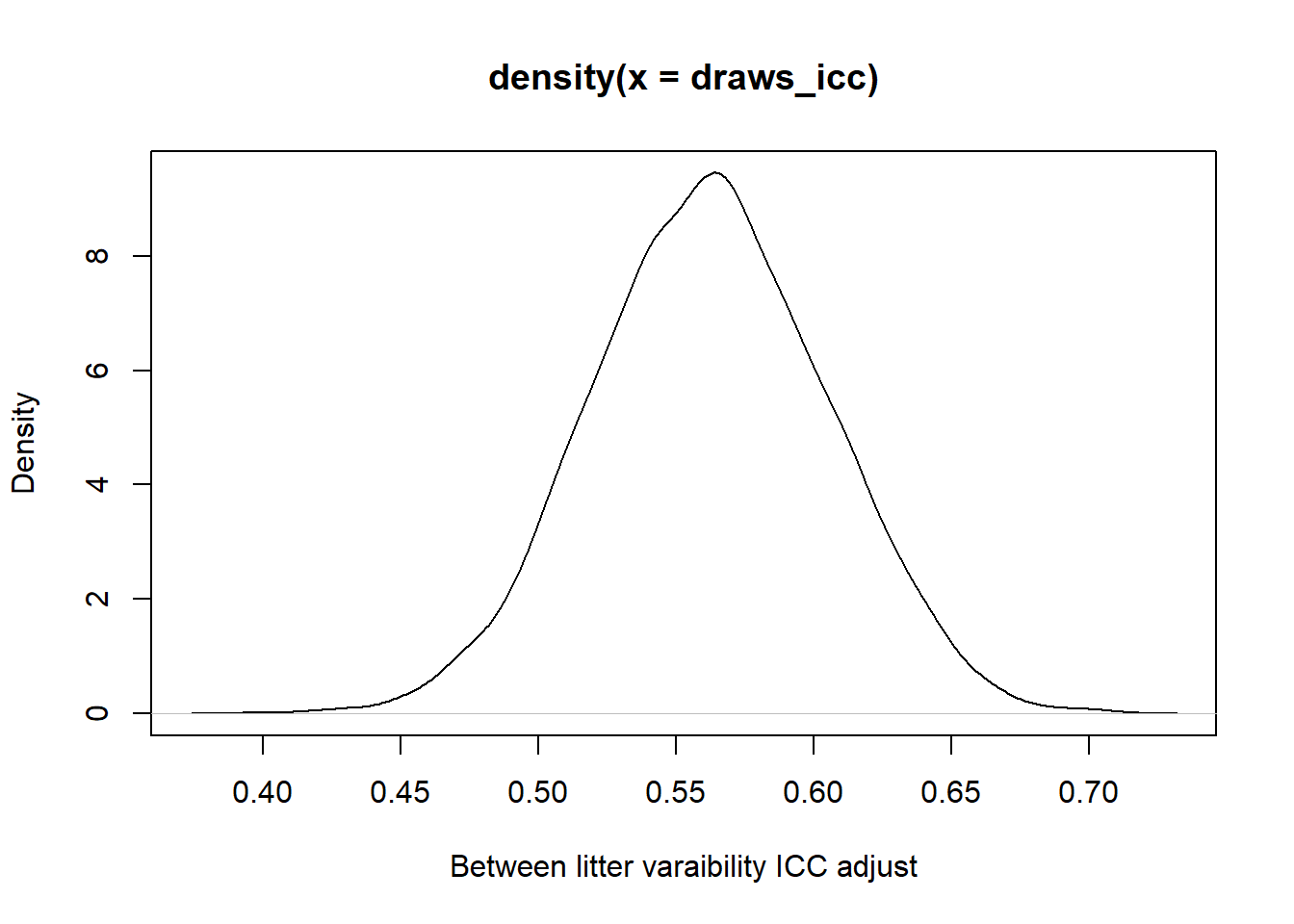
# Plot the adjusted ICC
plot(density(draws_icc), xlab = "Between litter varaibility ICC adjust")

It was estimated that 56%, 95% CI [48%, 65%] of the variations in fetal weight was attributed to between-litter differences.
We can use the posterior draws of b_Dose750, b_Dose1500, and b_Dose3000 (fix effects) to compute the posterior for the conditional ICC:

Code

# sjstats::icc(fit2) point estimate of adjusted and conditional ICC;
# Intraclass Correlation Coefficient
# 
#      Adjusted ICC: 0.565
#   Conditional ICC: 0.317

# calculating conditional ICC
post_par <- colMeans(posterior_samples(fit2, pars = c("b_Dose750","b_Dose1500","b_Dose3000")))
dummy <- with(ntp, outer(Dose, levels(Dose), `==`)*1)[,-1] #dummy matrix removing dose0 level;
sigma_f2 <- var(dummy%*%post_par)
draws_icc_conditional <- (draws_tau^2) / (draws_tau^2 + sigma_f2+ draws_sigma^2)
# quantile of posterior conditional ICC
quantile(draws_icc_conditional, p=c(0.5, 0.025,0.975))

      50%      2.5%     97.5% 
0.3138992 0.2497790 0.3913338

Code

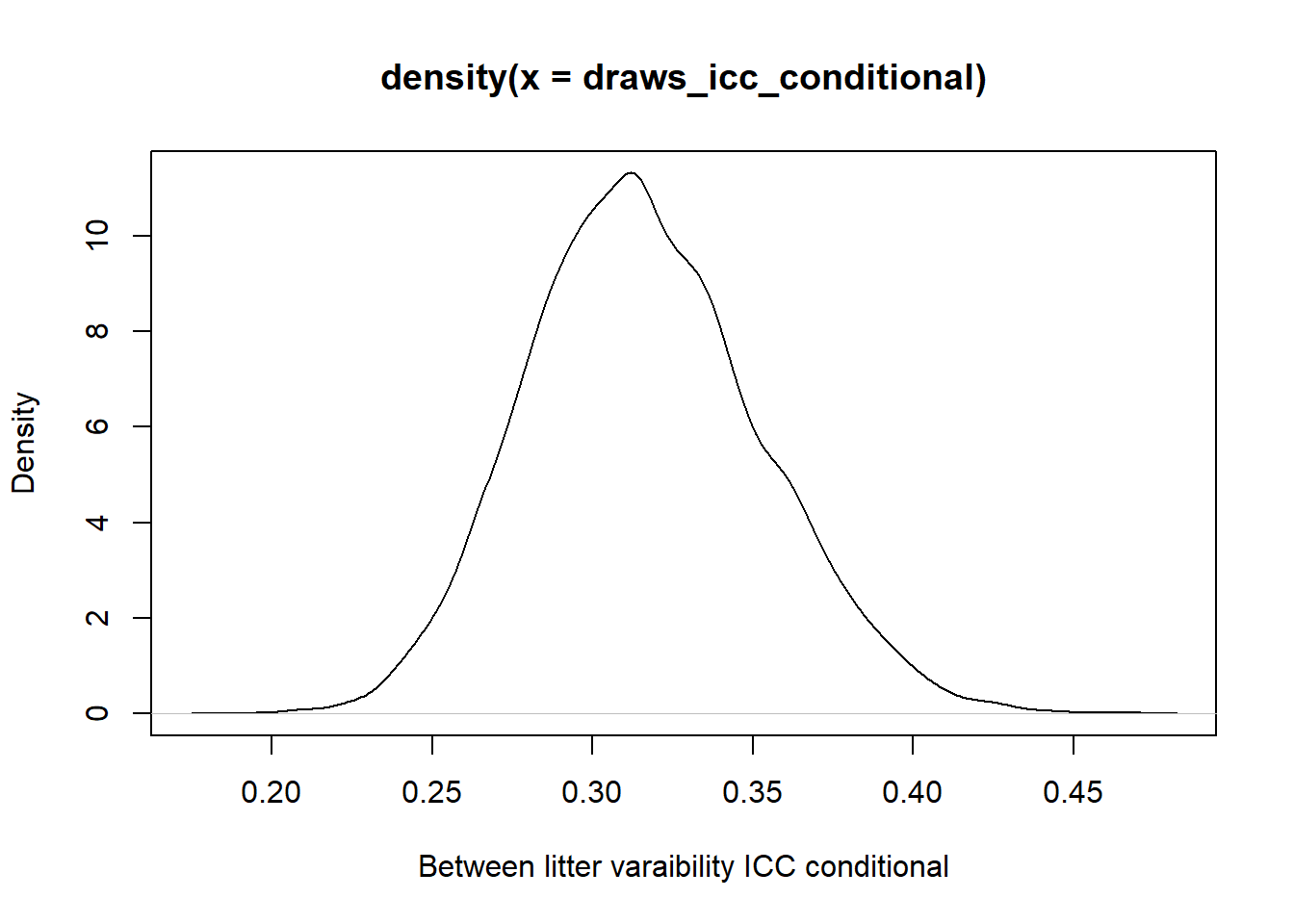
# Plot the adjusted ICC
plot(density(draws_icc_conditional), xlab = "Between litter varaibility ICC conditional")

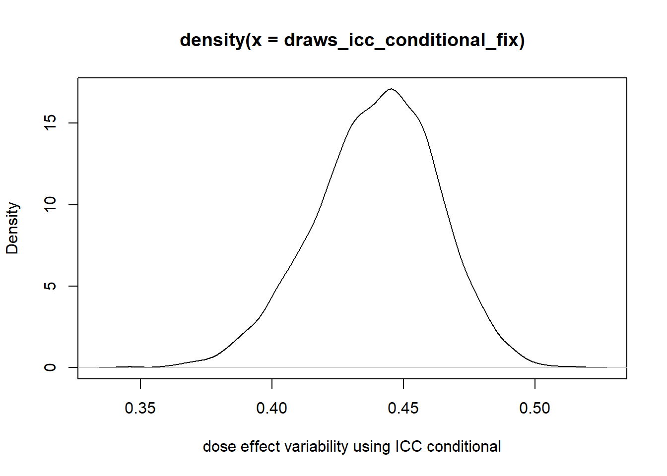
It was estimated that 31%, 95% CI [25%, 40%] of the variations in fetal weight was attributed to between-litter differences given fix effects.

Code

draws_icc_conditional_fix <- (sigma_f2) / (draws_tau^2 + sigma_f2+ draws_sigma^2)
# quantile of posterior conditional ICC
quantile(draws_icc_conditional_fix, p=c(0.5, 0.025,0.975))

      50%      2.5%     97.5% 
0.4409724 0.3906905 0.4821792

Code

# Plot the adjusted ICC
plot(density(draws_icc_conditional_fix), xlab = "dose effect variability using ICC conditional")

1.4 Normal hierarchical model with varying intercept and slope (model 2)

Variability in “velocity” between individual, dose the effect of dose on weight also vary by litter?
We want to build a model which recognizes that in the relationship between feta weight and dose,
- where the intercept (i.e., baseline weight)
- and slope (i.e., rate at which weight changes with dose) might vary from mouse to mouse.
A random intercept and slope model!
Variability within litter by dose
- in this model, \(\beta_{0j}\) and \(\beta_{1j}\) depend on litter
specifying our hierarchical random intercept and slope model :

\[ Y_{ij} \mid \beta_{0j}, \beta_{1j}, \sigma_y \sim N(\beta_{0j} + \beta_{1j} \ dose_{ij}, \sigma_y^2) \]

\[\beta_{0j} \mid \beta_{0}, \sigma_0^2\] \[\beta_{1j} \mid \beta_{1}, \sigma_1^2\]

In this model \(\beta_{0j}\) and \(\beta_{1j}\) working together to describe the model for litter \(j\), and thus are correlated!
Let \(\rho \in [-1,1]\) represents the correlation between \(\beta_{0j}\) and \(\beta_{1j}\). We can assign a joint Normal model of \(\beta_{0j}\) and \(\beta_{1j}\) where

\[ \begin{pmatrix} \beta_{0j}\\ \beta_{1j} \end{pmatrix} \mid \beta_{0}, \beta_{1}, \sigma_0, \sigma_1 \sim N(\begin{pmatrix} \beta_{0}\\ \beta_{1} \end{pmatrix}, \begin{pmatrix} \sigma_0^2 & \rho \sigma_0\sigma_1 \\ \rho \sigma_0\sigma_1 & \sigma_1^2 \end{pmatrix}). \]

\[\beta_{0} \sim N(0,10)\] \[\beta_{1} \sim N(0,10)\] \[\sigma_y \sim HalfCauchy(10)\] \[\sigma_0 \sim HalfCauchy(10)\] \[\sigma_1 \sim HalfCauchy(10)\] \[\mathbf{R} \sim LKJcorr(2)\]

where \(\mathbf{R}\) is the correlation matrix \[\begin{pmatrix} 1 & \rho \\ \rho & 1 \end{pmatrix}\]
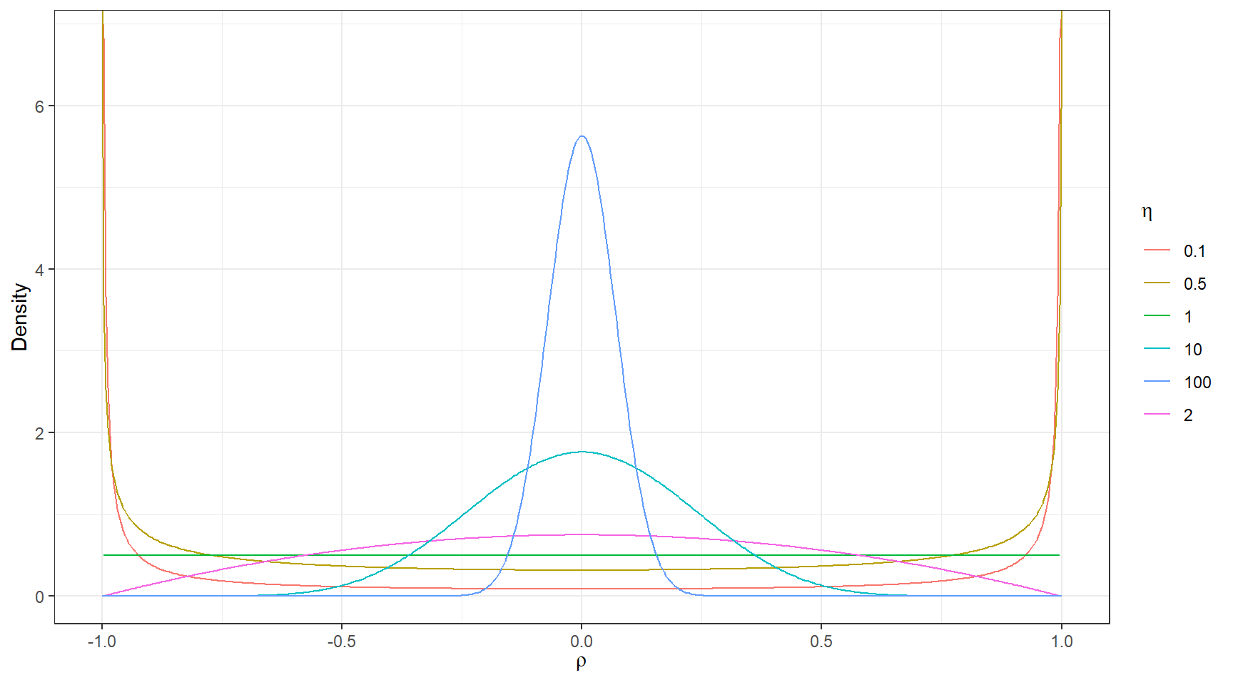
LKJ-correlation prior (Lewandowski, Kurowicka, and Joe 2009) with one parameter (\(\zeta\)) that controls the strength of the correlation.

Code

dlkjcorr2 <- function(rho, eta = 1, log = FALSE) {
  # Function to compute the LKJ density given a correlation
  out <- (eta - 1) * log(1 - rho^2) - 
    1 / 2 * log(pi) - lgamma(eta) + lgamma(eta + 1 / 2)
  if (!log) out <- exp(out)
  out
}
ggplot(tibble(rho = c(-1, 1)), aes(x = rho)) + 
  stat_function(fun = dlkjcorr2, args = list(eta = 0.1), 
                aes(col = "0.1"), n = 501) + 
  stat_function(fun = dlkjcorr2, args = list(eta = 0.5), 
                aes(col = "0.5"), n = 501) + 
  stat_function(fun = dlkjcorr2, args = list(eta = 1), 
                aes(col = "1"), n = 501) + 
  stat_function(fun = dlkjcorr2, args = list(eta = 2), 
                aes(col = "2"), n = 501) + 
  stat_function(fun = dlkjcorr2, args = list(eta = 10), 
                aes(col = "10"), n = 501) + 
  stat_function(fun = dlkjcorr2, args = list(eta = 100), 
                aes(col = "100"), n = 501) + 
  labs(col = expression(eta), x = expression(rho), y = "Density")+
  theme_bw()

LKJ prior for different values of the shape paramete

Code

fit3 <- brm(data = ntp,
            family= gaussian(),
            Weight ~ Dose + (Dose|Litter),  
            prior = c(prior(normal(0, 10), class = Intercept),
                      prior(normal(0, 10), class = b),
                      prior(cauchy(0, 10), class = sd),
                      prior(cauchy(0, 10), class = sigma),
                      prior(lkj(2), class = cor)),
            iter = 11000,
            warmup = 10000,
            chains = 3,
            cores = 4, 
            control = list(adapt_delta = .9), 
            seed = 123, 
            silent = 2,
            refresh = 0)
# saveRDS(fit3, "data/chp4_h_example3")

Posterior summary

Code

fit3 <- readRDS("data/chp4_h_example3")
summary(fit3)

 Family: gaussian 
  Links: mu = identity; sigma = identity 
Formula: Weight ~ Dose + (Dose | Litter) 
   Data: ntp (Number of observations: 1027) 
  Draws: 3 chains, each with iter = 11000; warmup = 10000; thin = 1;
         total post-warmup draws = 3000

Group-Level Effects: 
~Litter (Number of levels: 94) 
                        Estimate Est.Error l-95% CI u-95% CI Rhat Bulk_ESS
sd(Intercept)               0.07      0.01     0.05     0.09 1.01      385
sd(Dose750)                 0.05      0.03     0.00     0.13 1.01      300
sd(Dose1500)                0.07      0.04     0.00     0.15 1.01      334
sd(Dose3000)                0.08      0.04     0.01     0.16 1.01      254
cor(Intercept,Dose750)     -0.09      0.37    -0.73     0.67 1.00      635
cor(Intercept,Dose1500)    -0.02      0.35    -0.68     0.67 1.00      485
cor(Dose750,Dose1500)       0.01      0.38    -0.68     0.74 1.00      935
cor(Intercept,Dose3000)     0.02      0.36    -0.67     0.71 1.00      500
cor(Dose750,Dose3000)       0.01      0.38    -0.70     0.72 1.00      713
cor(Dose1500,Dose3000)      0.02      0.38    -0.70     0.72 1.01      804
                        Tail_ESS
sd(Intercept)               1063
sd(Dose750)                  671
sd(Dose1500)                 797
sd(Dose3000)                 388
cor(Intercept,Dose750)       785
cor(Intercept,Dose1500)      572
cor(Dose750,Dose1500)       1527
cor(Intercept,Dose3000)      799
cor(Dose750,Dose3000)       1173
cor(Dose1500,Dose3000)      1491

Population-Level Effects: 
          Estimate Est.Error l-95% CI u-95% CI Rhat Bulk_ESS Tail_ESS
Intercept     0.97      0.01     0.95     1.00 1.00      842     1310
Dose750      -0.09      0.02    -0.14    -0.05 1.00     1276     1748
Dose1500     -0.19      0.03    -0.25    -0.14 1.00     1387     1757
Dose3000     -0.26      0.03    -0.32    -0.21 1.00     1500     1921

Family Specific Parameters: 
      Estimate Est.Error l-95% CI u-95% CI Rhat Bulk_ESS Tail_ESS
sigma     0.07      0.00     0.07     0.08 1.00     3616     2306

Draws were sampled using sampling(NUTS). For each parameter, Bulk_ESS
and Tail_ESS are effective sample size measures, and Rhat is the potential
scale reduction factor on split chains (at convergence, Rhat = 1).

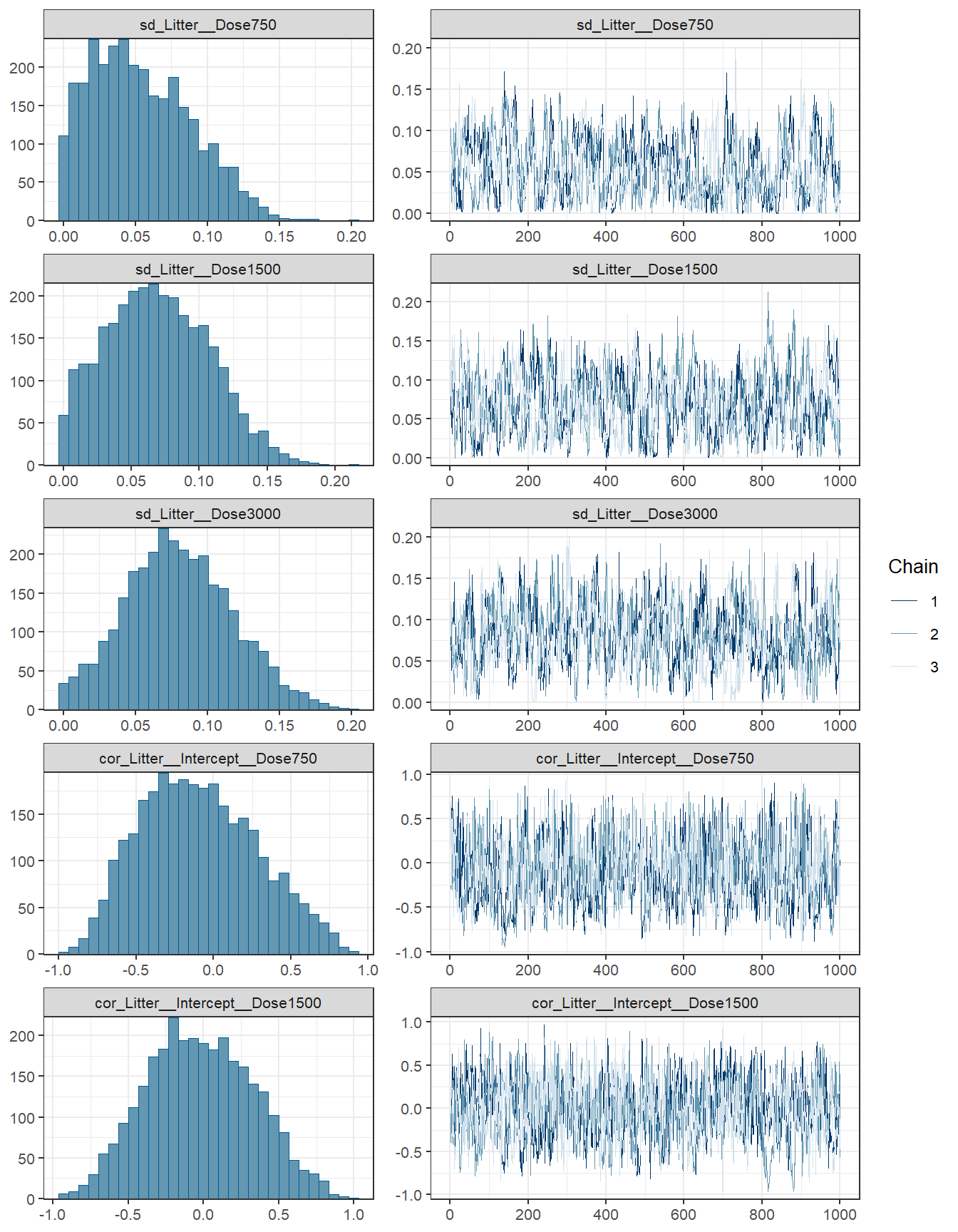
Code

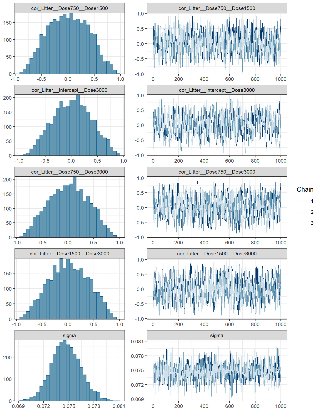
fit3 %>% plot( combo = c("hist", "trace"), widths = c(1, 1.5),
      theme = theme_bw(base_size = 10))

Code

conditional_effects(fit3)

Interpretations
- Example interpretation for does750, “Moving from 0 to 750 dose is associated with a mean weight decrease of 0.09 units. Credible interval excludes 0 indicating a strong evidence of a negative effect.”
- Example interpretation for sd(Intercept), “Typical litters differ in baseline weight by rouhgly \(\pm\) 0.07 units around the group mean weight of 0.97 for dose 0.”
- Example interpretation for sd(Dose 750)), “Litter-specific 750 dosing effect varies rouhgly \(\pm\) 0.05 units around the group mean weight for dose 750”
- Interpretation for sigma, variability of individual weights around their litter- and dose-specific mean. This is the “left-over” noise once fixed and random effects are accounted for.

Comparing between the two models
elpd difference is less than 4 indicating the two models are very similar in fit.

Code

loo1 <- loo(fit2)
loo2 <- loo(fit3)
loo_compare(loo1, loo2)

     elpd_diff se_diff
fit3  0.0       0.0   
fit2 -0.3       1.1

Comparing between the random intercept and random slope models
- Random intercept only: baseline weight varies; dose effects are the same for all litters; Litters differ only in starting weights;
- Random slope: baseline weight and dose effects vary by litter; Some litters are more/less sensitive to dosing effect.
- Model choice:
  - Statistical implication: Given LOO results, there is no evidence that the random-slope model predicts new data better than the simpler random-intercept model.
  - Practical implication: Unless scientific reasoning requires slope heterogeneity, favor fit2 for parsimony (fewer parameters, faster computation, easier interpretation).

1.5 Hierarchical model with a binary outcome

Let’s look at a hospital mortality study as an example. This data capture hospital mortality for a specific condition at 20 different hospitals. There is also a variable that describes the average severity of patients at each hospital.

First let’s examine the data

Code

dat <- read.table("data/HospitalMortality.csv",sep=",", header=T)

dat <- dat %>% 
  mutate(Hospital = factor(Hospital),
         Prop.Dead = round(Deaths/N,3))

dat %>% datatable(
  rownames = FALSE,
  options = list(
    columnDefs = list(list(className = 'dt-center', 
                      targets = 0:4))))

Code

dat %>% select(Severity, Prop.Dead) %>% tbl_summary()

Characteristic	N = 25¹
Severity	4.10 (3.60, 4.60)
Prop.Dead	0.05 (0.04, 0.08)
¹ Median (IQR)

1. First model - considering independent between hospital mortality

We are modelling \[Death_i \sim Bin(p_i, n_i)\], where \(i = 1, \ldots, 25\) and \(p_i\) represent the risk of death for the \(i\) hospital with a beta(1,1) prior on all \(p_i\)s
This model is saying that there is nothing to link mortality in hospital 1 to mortality in any other hospital
- We are essentially estimating the risk of mortality for each hospital

Code

fit1 <- brm(data = dat,
            family= binomial,
            Deaths | trials(N) ~ 0 + Hospital,  
            iter = 10000,
            warmup = 8000,
            chains = 4,
            cores = 4, 
            seed = 123, 
            silent = 2,
            refresh = 0)
# saveRDS(fit1, "data/chp4_h_example1")

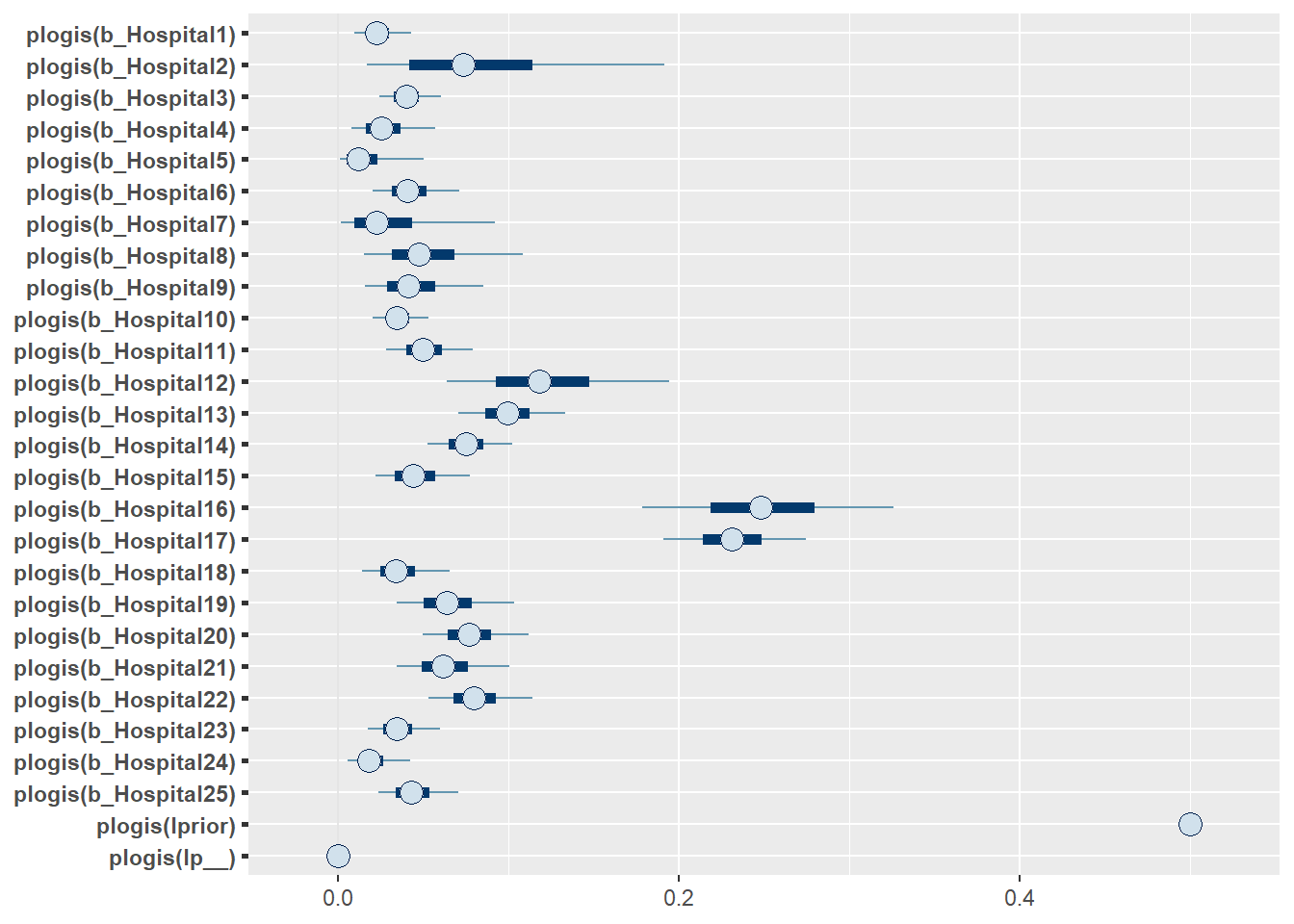
Summarizing posterior results

Code

fit1 <- readRDS("data/chp4_h_example1")
summary(fit1)

 Family: binomial 
  Links: mu = logit 
Formula: Deaths | trials(N) ~ 0 + Hospital 
   Data: dat (Number of observations: 25) 
  Draws: 4 chains, each with iter = 10000; warmup = 8000; thin = 1;
         total post-warmup draws = 8000

Population-Level Effects: 
           Estimate Est.Error l-95% CI u-95% CI Rhat Bulk_ESS Tail_ESS
Hospital1     -3.81      0.47    -4.82    -3.00 1.00     9872     5377
Hospital2     -2.63      0.82    -4.48    -1.26 1.00    11409     5289
Hospital3     -3.19      0.28    -3.79    -2.67 1.00    11066     5403
Hospital4     -3.72      0.63    -5.11    -2.67 1.00    10042     4824
Hospital5     -4.65      1.30    -7.74    -2.74 1.00     9267     4313
Hospital6     -3.18      0.40    -4.02    -2.47 1.00    12339     5584
Hospital7     -3.98      1.27    -6.93    -2.06 1.00     8965     4235
Hospital8     -3.05      0.63    -4.48    -1.98 1.00     9535     4484
Hospital9     -3.19      0.55    -4.37    -2.24 1.00    10237     5257
Hospital10    -3.35      0.30    -3.99    -2.80 1.00    11680     5665
Hospital11    -2.97      0.34    -3.68    -2.37 1.00    11899     6003
Hospital12    -2.03      0.39    -2.83    -1.33 1.00     9612     5937
Hospital13    -2.21      0.22    -2.65    -1.80 1.00    11803     5516
Hospital14    -2.52      0.22    -2.97    -2.11 1.00    11147     6079
Hospital15    -3.10      0.41    -3.96    -2.38 1.00    12498     5485
Hospital16    -1.12      0.24    -1.60    -0.66 1.00    11560     6024
Hospital17    -1.20      0.14    -1.48    -0.93 1.00    10363     6579
Hospital18    -3.39      0.48    -4.44    -2.55 1.00    10986     5471
Hospital19    -2.71      0.36    -3.45    -2.07 1.00    11680     6152
Hospital20    -2.50      0.27    -3.04    -2.00 1.00    10498     6086
Hospital21    -2.74      0.35    -3.46    -2.10 1.00    11060     6154
Hospital22    -2.46      0.25    -2.98    -1.98 1.00    12458     5873
Hospital23    -3.36      0.40    -4.20    -2.65 1.00    10596     5825
Hospital24    -4.06      0.63    -5.44    -2.99 1.00    10608     5415
Hospital25    -3.12      0.35    -3.87    -2.48 1.00    11722     5842

Draws were sampled using sampling(NUTS). For each parameter, Bulk_ESS
and Tail_ESS are effective sample size measures, and Rhat is the potential
scale reduction factor on split chains (at convergence, Rhat = 1).

Code

#posterior summary of risk (table);
round(exp(fixef(fit1)),3)

           Estimate Est.Error  Q2.5 Q97.5
Hospital1     0.022     1.596 0.008 0.050
Hospital2     0.072     2.273 0.011 0.283
Hospital3     0.041     1.329 0.023 0.069
Hospital4     0.024     1.875 0.006 0.069
Hospital5     0.010     3.663 0.000 0.065
Hospital6     0.042     1.485 0.018 0.084
Hospital7     0.019     3.561 0.001 0.128
Hospital8     0.047     1.884 0.011 0.138
Hospital9     0.041     1.725 0.013 0.107
Hospital10    0.035     1.351 0.019 0.061
Hospital11    0.051     1.399 0.025 0.094
Hospital12    0.132     1.475 0.059 0.266
Hospital13    0.109     1.241 0.071 0.165
Hospital14    0.080     1.247 0.051 0.121
Hospital15    0.045     1.504 0.019 0.092
Hospital16    0.328     1.275 0.201 0.519
Hospital17    0.300     1.153 0.227 0.395
Hospital18    0.034     1.619 0.012 0.078
Hospital19    0.066     1.429 0.032 0.127
Hospital20    0.082     1.305 0.048 0.135
Hospital21    0.065     1.415 0.031 0.122
Hospital22    0.086     1.289 0.051 0.138
Hospital23    0.035     1.485 0.015 0.071
Hospital24    0.017     1.885 0.004 0.050
Hospital25    0.044     1.425 0.021 0.084

Code

#posterior summary of risk (visual);
mcmc_intervals(fit1, transformations = "plogis")

2. Second model - shared parameters on hospital mortality (complete pooling)

Suppose that these were 25 hospitals in the same city
- Similar practices, populations, shared staff in some cases
How can we treat them as one big hospital with exactly the same mortality?
- Easy - specify in the model that they share the same probability \(p\)
Parameterizing using odds
- Odds are the basis for logistic regression, where we model log(odds)
- \(0 \leq p \leq 1 \Rightarrow - \infty \leq \log(Odds) \leq \infty\)
- Suggests an normal uninformative prior on log odds with a sufficient variance (ie sd = 10)
\[ \log(Odds) \sim N(0,\sigma^2)\]
Assume a common odds between all 25 hospitals, we run a pooled model such that \[Death_i \sim Bin(p, n_i)\]. This is a complete pooling model.
We are essentially modelling the average population risk of mortality pooling information from all 25 hospitals.

Code

fit1.p <- brm(data = dat,
            family= binomial,
            Deaths | trials(N) ~ 1,  
            iter = 10000,
            warmup = 8000,
            chains = 4,
            cores = 4, 
            seed = 123, 
            silent = 2,
            refresh = 0)
# saveRDS(fit1.p, "data/chp4_h_example1p")

Summarizing posterior results

 Family: binomial 
  Links: mu = logit 
Formula: Deaths | trials(N) ~ 1 
   Data: dat (Number of observations: 25) 
  Draws: 4 chains, each with iter = 10000; warmup = 8000; thin = 1;
         total post-warmup draws = 8000

Population-Level Effects: 
          Estimate Est.Error l-95% CI u-95% CI Rhat Bulk_ESS Tail_ESS
Intercept    -2.60      0.06    -2.72    -2.48 1.00     2774     3505

Draws were sampled using sampling(NUTS). For each parameter, Bulk_ESS
and Tail_ESS are effective sample size measures, and Rhat is the potential
scale reduction factor on split chains (at convergence, Rhat = 1).

          Estimate Est.Error  Q2.5 Q97.5
Intercept    0.074     1.063 0.066 0.084

Drawbacks of a complete pooling approach

There are two main drawbacks to taking a complete pooling approach to analyze group structured data:

in case of clustered and correlated data, we violate the assumption of independence
misleading conclusions about the relationship between and across subjects

3. third model - shared parameters on hospital mortality (partial pooling)

Suppose that these were 25 hospitals in the same city
- Similar (but not same) practices and patient populations; partly shared staff
How can we treat them as similar
- with a common underlying true mortality
- with random variation from hospital to hospital in the true mortality!
Need to introduce two parameters representing
- Common mortality (mean log odds)
- Hospital-to-hospital variation (sd of log odds)
This introduces an hierarchical structure in the model!
Specifically, we have
1. Data Layer \(y_i \mid p_i \sim P(y_i \mid p_i)\)
2. Adaptive/Structural Priors \(logit(p_i) \mid \theta, \sigma^2 \sim P(logit(p_i) \mid \theta, \sigma^2)\)
3. Hyper Priors \(\theta \sim P(\theta)\) and \(\sigma^2 ~ P(\sigma^2)\) as hyper parameters.
A Bayesian random intercept model!

Code

fit1.ri <- brm(data = dat,
            family= binomial,
            Deaths | trials(N) ~ 1 + (1|Hospital),  
            iter = 10000,
            warmup = 8000,
            chains = 4,
            cores = 4, 
            seed = 123, 
            silent = 2,
            refresh = 0)
# saveRDS(fit1.ri, "data/chp4_h_example1ri")

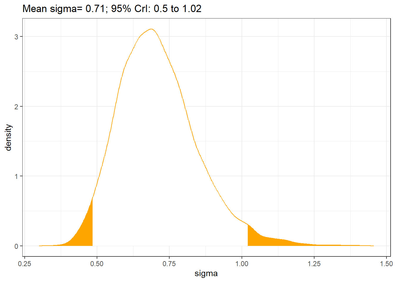
Summarizing posterior results on risk and between-hospital standard deviation of the intercept

Code

fit1.ri <- readRDS("data/chp4_h_example1ri")
prior_summary(fit1.ri)

                prior     class      coef    group resp dpar nlpar lb ub
 student_t(3, 0, 2.5) Intercept                                         
 student_t(3, 0, 2.5)        sd                                     0   
 student_t(3, 0, 2.5)        sd           Hospital                  0   
 student_t(3, 0, 2.5)        sd Intercept Hospital                  0   
       source
      default
      default
 (vectorized)
 (vectorized)

Code

summary(fit1.ri)

 Family: binomial 
  Links: mu = logit 
Formula: Deaths | trials(N) ~ 1 + (1 | Hospital) 
   Data: dat (Number of observations: 25) 
  Draws: 4 chains, each with iter = 10000; warmup = 8000; thin = 1;
         total post-warmup draws = 8000

Group-Level Effects: 
~Hospital (Number of levels: 25) 
              Estimate Est.Error l-95% CI u-95% CI Rhat Bulk_ESS Tail_ESS
sd(Intercept)     0.71      0.14     0.48     1.02 1.00     2272     3574

Population-Level Effects: 
          Estimate Est.Error l-95% CI u-95% CI Rhat Bulk_ESS Tail_ESS
Intercept    -2.81      0.17    -3.16    -2.49 1.00     2160     3428

Draws were sampled using sampling(NUTS). For each parameter, Bulk_ESS
and Tail_ESS are effective sample size measures, and Rhat is the potential
scale reduction factor on split chains (at convergence, Rhat = 1).

Code

#posterior summary of risk overall (table);
round(exp(fixef(fit1.ri)),3)

          Estimate Est.Error  Q2.5 Q97.5
Intercept     0.06     1.185 0.043 0.083

Code

s1 <- posterior_samples(fit1.ri)
sigma <- s1[,"sd_Hospital__Intercept"]
qs <- quantile(sigma,c(0.025, 0.975))

temp <- density(sigma,n = 1024)
dp1 <- data.frame(sigma=temp$x, density=temp$y, area=cut(temp$x, c(0,qs,10), include.lowest = T))

ggplot(dp1, aes(x=sigma, y=density))+geom_area(aes(fill=area), show.legend=FALSE)+
    theme_bw()+
    geom_line(color="orange")+
    ggtitle(paste0("Mean sigma= ", round(mean(sigma),2),"; 95% CrI: ", round(qs[1],1),
                   " to ",round(qs[2],2)))+
    scale_fill_manual(values=c("orange","white","orange"))

Hospitals, ranked best to worst by posterior odds of mortality (median ranking on mortality, along with a 95% CrI)

Code

h <- s1[,grep(",Intercept",names(s1))]
r <- apply(h,1,rank)
rankings <- t(apply(r,1,quantile, c(0.5, c(0.025, 0.975))))
row.names(rankings) <- paste("Hospital",1:25)
colnames(rankings)[1] <- "Median"
rankings <- data.frame(rankings, ObservedProportion=round(dat$Deaths/dat$N,3), n=dat$N)
rankings <- rankings[order(rankings[,1]),]
knitr::kable(rankings, caption="Hospitals, ranked best to worst by posterior odds of mortality")

Hospitals, ranked best to worst by posterior odds of mortality
	Median	X2.5.	X97.5.	ObservedProportion	n
Hospital 24	3	1	15	0.020	149
Hospital 1	4	1	14	0.024	209
Hospital 5	5	1	19	0.017	60
Hospital 4	6	1	18	0.028	109
Hospital 10	7	1	15	0.035	340
Hospital 18	8	1	19	0.036	140
Hospital 23	8	1	17	0.036	196
Hospital 3	9	2	17	0.041	319
Hospital 6	10	2	19	0.043	164
Hospital 7	10	1	22	0.031	32
Hospital 25	10	2	19	0.044	203
Hospital 9	11	1	21	0.045	89
Hospital 15	11	2	20	0.046	153
Hospital 11	12	3	20	0.051	196
Hospital 8	13	2	23	0.053	57
Hospital 19	16	5	22	0.065	138
Hospital 21	16	4	22	0.063	142
Hospital 2	17	2	23	0.083	24
Hospital 14	18	11	23	0.076	290
Hospital 20	19	10	23	0.078	192
Hospital 22	19	11	23	0.081	211
Hospital 12	22	12	23	0.123	65
Hospital 13	22	16	23	0.100	250
Hospital 16	24	24	25	0.250	92
Hospital 17	25	24	25	0.232	267

comparing models
- Model 3 has the best fit!

Code

loo1 <- loo(fit1)
loo2 <- loo(fit1.p)
loo3 <- loo(fit1.ri)
loo_compare(loo1, loo2, loo3)

        elpd_diff se_diff
fit1.ri   0.0       0.0  
fit1     -7.7       2.5  
fit1.p  -62.4      38.9

References

Bürkner, Paul-Christian. 2017. “Advanced Bayesian Multilevel Modeling with the r Package Brms.” arXiv Preprint arXiv:1705.11123.

Lewandowski, Daniel, Dorota Kurowicka, and Harry Joe. 2009. “Generating Random Correlation Matrices Based on Vines and Extended Onion Method.” Journal of Multivariate Analysis 100 (9): 1989–2001.

Nakagawa, Shinichi, Paul CD Johnson, and Holger Schielzeth. 2017. “The Coefficient of Determination r 2 and Intra-Class Correlation Coefficient from Generalized Linear Mixed-Effects Models Revisited and Expanded.” Journal of the Royal Society Interface 14 (134): 20170213.

Price, Catherine J, Carole A Kimmel, Rochelle W Tyl, and Melissa C Marr. 1985. “The Developmental Toxicity of Ethylene Glycol in Rats and Mice.” Toxicology and Applied Pharmacology 81 (1): 113–27.