require(tidyverse)
library(cowplot)Tutorial 2
1. Hands-on excerise Working with Beta-binomail model
Learning objectives:
- Plotting beta densities (prior and posterior) in R (review from tutorial 1)
- Understand how we can update posterior belief with new data under Bayesian framework
- Learn how to use posterior probabilities for statistical and clinical inference
Example
Suppose we are running a single arm phase I safety study of a new drug A.
- (Clinical relevant target) We define aprior an adverse event (AE) rate above 30% as unacceptable.
- (clinical decision) If there is statistical evidence that we have at least 90% certainty that the AE rate is < 30%, we will stop the trial early.
Let \(\theta\) represents the true AE rate for drug A and we are interested in estimating \(\theta\) using the Beta-binomial Bayesian model.
- Step 1. Deciding on a reasonable prior
- Let’s say we have two candidate priors, Beta(1,1) and Beta (2,8). Please plot the two beta distributions in R (review from tutorial 1).
- what would you comment about the two priors?
- hint: if \(\theta \sim Beta(\alpha, \beta)\), \(E[\theta] = \frac{\alpha}{\alpha+\beta}\).
# we can create a R function to efficiently generate plots;
beta_plot <- function(shape1=1, shape2=1){
  # creating x vector;
x <- seq(from = 0, to = 1, by = 0.001)
# finding density probability for each x element;
y <- dbeta(x, shape1 = shape1, shape2 = shape2)
# create a plotting dataframe;
data <- data.frame(x,y)
# ggplot;
ggplot(data, aes(x=x, y=y)) +
  geom_line() +
  labs(x='X', y='density', title=paste0('Beta(',shape1,',',shape2,')'))+
  theme_bw()
}

p1<-beta_plot(1,1)
p2<-beta_plot(2,8)
plot_grid(p1, p2, labels = c('A', 'B'), label_size = 12)
- Step 2. Getting data. Suppose we enrolled three participants to our trial, all received drug A, and no one experienced AE.
- what is the observed AE in this sample of 3? 0% < 30%.
- Step 3. Derive posterior distribution given data and prior. Suppose we choose Beta(1,1) as our prior belief for \(\theta\). Given what you have learned in the class today, what is the posterior distribution?
- Note that \(\theta_0 \sim Beta(1,1)\) and among the \(n=3\) samples we have \(X=0\) and \(n-x=3\)
- Please calculate the posterior distribution.
Posterior distribution
beta_plot(1,4)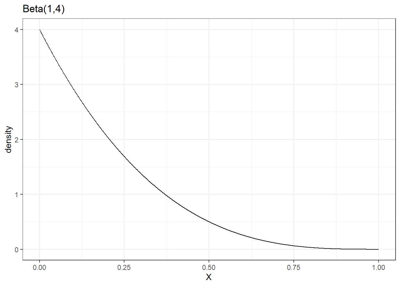
- Step 4. Making inference with posterior distribution. We are interested to know what is probability for \(P(\theta < 0.3)\).
Making posterior inference directly from pbeta()
pbeta(0.3, shape1 = 1, shape2 = 4, lower.tail = TRUE)[1] 0.7599what can you conclude? Do you believe the true AE rate is less than 30%? Can we stop the trial?
Step 6. We enrolled another 3 patients and none of them experienced AE. What is your updated belief?
- We treat the earlier updated belief (posterior distribution) as the new prior!
- \(\theta_0 \sim Beta(1,4)\) and among the \(n=3\) samples we have \(X=0\) and \(n-x=3\).
- What is the updated \(P(\theta < 0.3)\)? And your conclusion?
- Can we stop the trial?
Updated posterior distribution
beta_plot(1,7)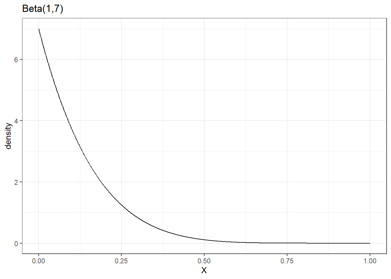
pbeta(0.3, shape1 = 1, shape2 = 7, lower.tail = TRUE)[1] 0.9176457
Making posterior inference using monte carlo methods via repeated sampling from the posterior distribution
# we generate 10000 random samples from the posterior Beta distribution;
num.samples <- 10000
theta.samples <- rbeta(num.samples, shape1 = 1, shape2 = 4)
plot(density(theta.samples))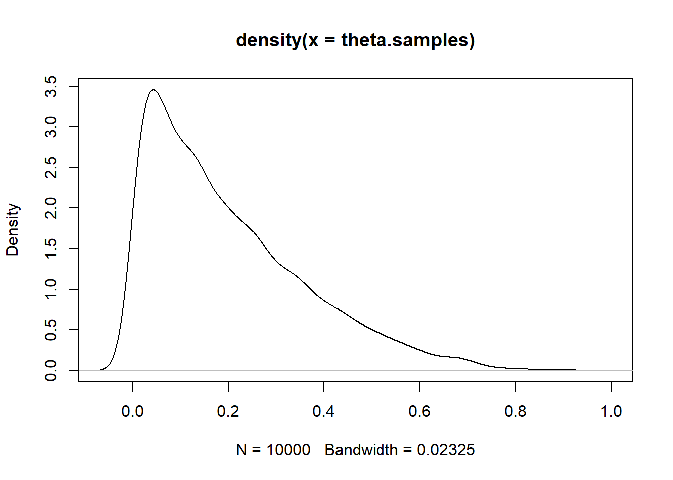
# calculating proportion of theta samples among the 1000 draws that are larger than 0.3;
sum(theta.samples < 0.3)/num.samples
[1] 0.7609mean(theta.samples < 0.3) #another way of estimating the same probability;[1] 0.7609