Tutorial 3

require(tidyverse)
library(extraDistr)

Hands-on exercise on prior elicitation

1. The BIPED Study

Project: Remote expert elicitation to determine the prior probability distribution for Bayesian sample size determination in international randomized controlled trials: Bronchiolitis in Infants Placebo Versus Epinephrine and Dexamethasone (BIPED) Study

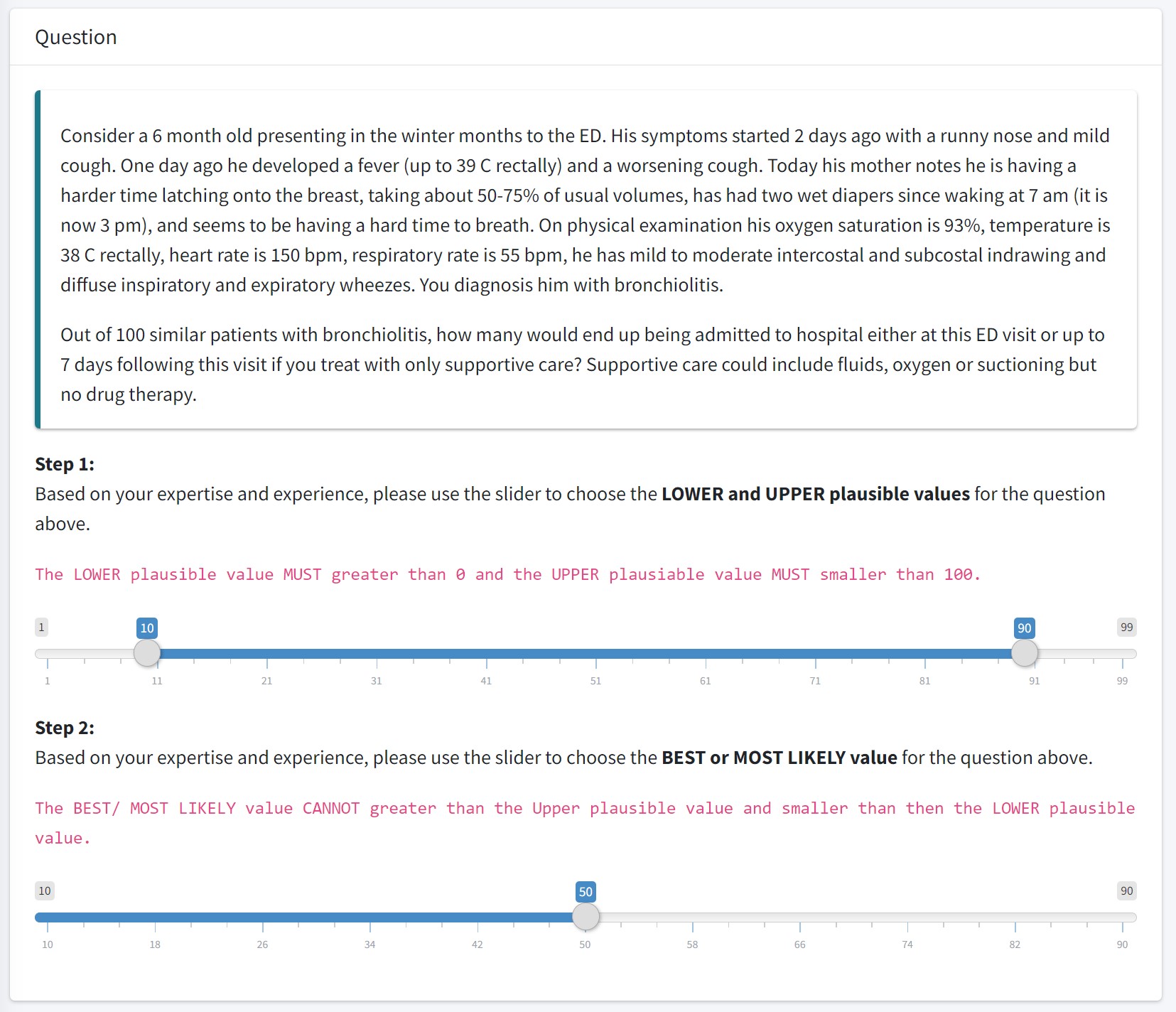
BIPED study prior elicitation individual response distribution

1.1 Given a range of beliefed pausible value, how can we calculate beta distribution parameters?

Mathematically, we are solving for \(\alpha\) and \(\beta\) given L and U and the mode (“best value”);

\[P(L < \theta < U) = 0.95\] \[\theta \sim Beta(\alpha, \beta)\] - Let \(\theta\) be the number of patient end up being admitted to hospital out of 100 similar patients with bronchiolitis

Suppose expert A pick the range as [10,90], that is \(P(10<\theta<90)=0.95\) and if we assume \(\theta\) follows a Beta distribution, and the mode, \(50 = \frac{\alpha-1}{\alpha+\beta-2}\) can we find the corresponding \(\alpha\) and \(\beta\) of this beta distribution?
- Given 95% CR, how to reverse calculation to get Beta distribution parameters: alpha and beta;
We can use maximum likelihood estimation (MLE)! A statistical estimation method that helps us to identify a parametric distribution using empirical percentile.

# For this calculation we want to use beta-binomial distribution;
# This is because the confidence region in the BIPED app is reported on the number of events out of 100 standard patients.
# let's write out the likelihood of beta-binomial model

expert_beta <- function(L, U, mode, level = 0.95) {
  stopifnot(0 < L, L < U, U < 1,
            0 < mode, mode < 1,
            level > 0, level < 1)

  # One-dimensional objective: log-k keeps the search on (0,???)
  objective <- function(logk) {
    k      <- exp(logk)
    alpha  <- 1 + mode * k
    beta   <- 1 + (1 - mode) * k
    q_low  <- qbeta( (1 - level)/2, alpha, beta )
    q_high <- qbeta( 1 - (1 - level)/2, alpha, beta )
    (q_low  - L)^2 + (q_high - U)^2
  }

  opt <- optimize(objective, interval = c(-15, 25))   # log-scale search
  k   <- exp(opt$minimum)
  list(alpha = 1 + mode * k,
       beta  = 1 + (1 - mode) * k,
       SSE   = opt$objective)          # residual mis-fit (???0 if feasible)
}

# Maximize the likelihood using optim function;
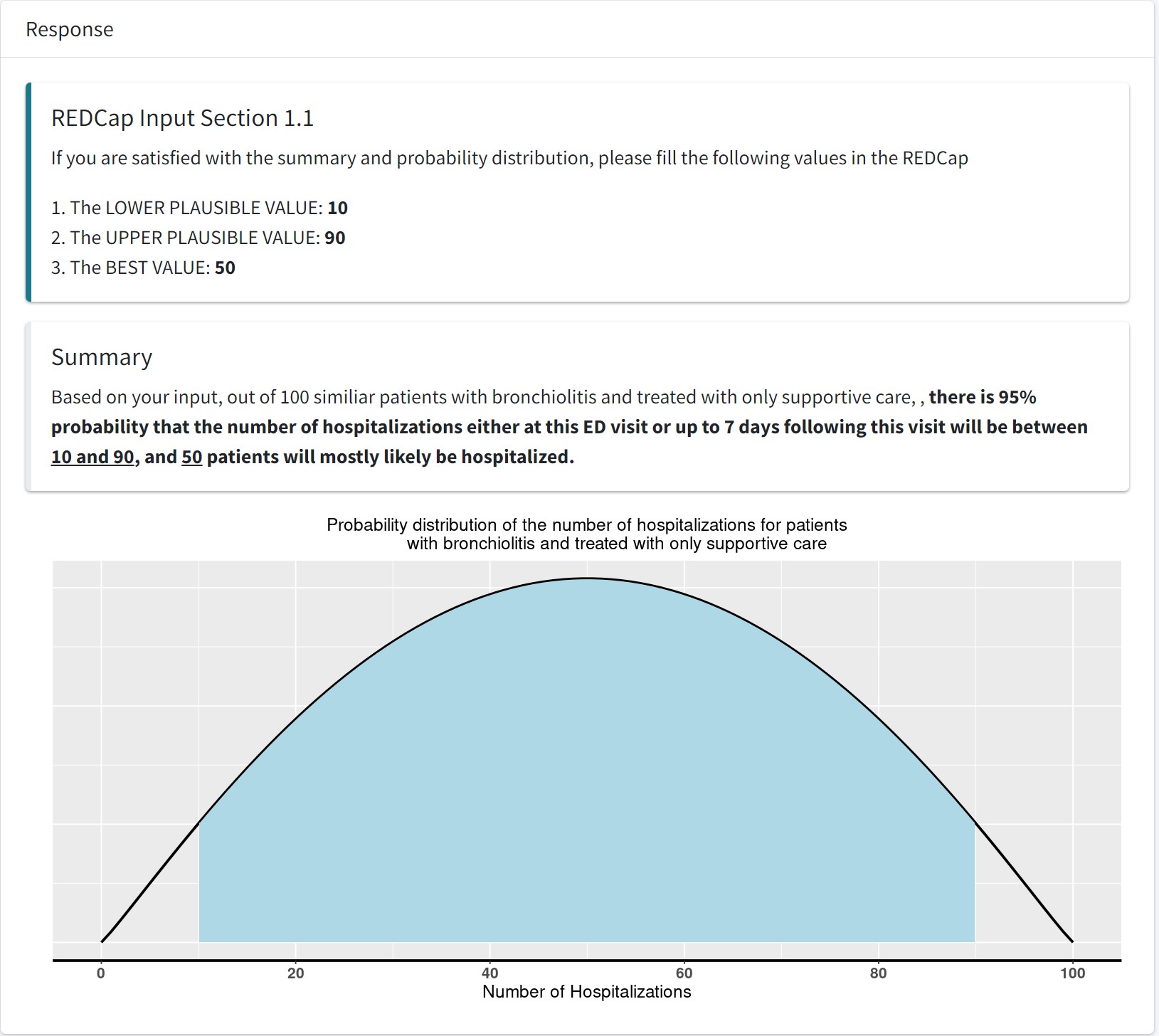
expert_beta(L = 10/100, U = 90/100, mode = 50/100)

$alpha
[1] 2.093438

$beta
[1] 2.093438

$SSE
[1] 4.746533e-15

Expert A selected a \(Beta(\alpha = 2.093438, \beta = 2.093438)\)

# we can create a R function to efficiently generate plots;
beta_plot <- function(shape1=1, shape2=1, scale = 100){
  # creating x vector;
x <- seq(from = 0, to = 1, by = 0.001)
# finding density probability for each x element;
y <- dbeta(x, shape1 = shape1, shape2 = shape2)
# create a plotting dataframe;
data <- data.frame(x,y)
# ggplot;
ggplot(data, aes(x=x*scale, y=y)) +
  geom_line() +
  labs(x=bquote(.(scale) * theta), y='density', title=paste0('Beta(',shape1,',',shape2,')'))+
  theme_bw() 
}

beta_plot(2.093438,2.093438)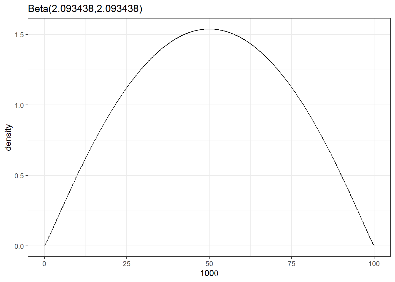

What is the expected number of hospitalization? (mean of the beta distribution)

\[100 \times \frac{2.093438}{2.093438+2.093438} = 50 \]

Suppose expert B pick the range as [50,90] and mode 80, what is expert B’s Beta distribution?

beta_parameters<-expert_beta(L = 50/100, U = 90/100, mode = 80/100)

beta_plot(beta_parameters$alpha,beta_parameters$beta)

mean = 100*(beta_parameters$alpha/(beta_parameters$alpha+beta_parameters$beta))
mean

[1] 75.61505

1.2 Combine multiple expert options - (pooled) mixture distribution

a1 <- 2.09
b1 <- 2.09

a2 <- 10.35
b2 <- 3.34

w  <- c(1/2,1/2) #assign equal mixture weight to the two believes;

theta <- seq(0,1,0.01)
p1 <- dbeta(theta,a1,b1)
p2 <- dbeta(theta,a2,b2)

pool <- w[1]*p1+w[2]*p2

r  <- 1.2*max(c(p1,p2, pool))

plot(theta,p1,col=gray(0.5),lwd=2,ylim=c(0,r),type="l",
     xlab=expression(theta),ylab="Prior",
     cex.lab=1.5,cex.axis=1.5)
lines(theta,p2,col=gray(0.5),lwd=2)
lines(theta,pool,col="red",lwd=2)
legend("topleft",c("Experts","Mixture of experts"),lwd=2,col=c(gray(0.5), "red"),bty="n",cex=1.5)

2. Specifying a skeptical prior for log-OR

In clinical trials, effect sizes are often expressed as an odds ratio (OR). As discussed in the lecture, prior distributions for OR are specified on the log(OR) scale, where a normal distribution is appropriate since log-transformed estimates are approximately normally distributed.

A common clinical prior is the skeptical prior: a normal distribution centered at OR = 1 (no effect, i.e., \(\log(1) = 0\)), with the spread chosen to reflect doubt about large treatment effects.

2.1 Finding the prior SD from a credible interval statement

Suppose a clinical expert states:

“A skeptical prior should be a normal distribution centred at an OR of 1 with approximately a 50% probability of an OR between 0.8 and 1.25.”

This region (0.8 to 1.25) is often called the similarity region the range where the treatment effect would be considered clinically negligible.

We need to find \(\sigma\) for \(\log(OR) \sim N(0, \sigma^2)\) such that:

\[P(\log(0.8) < \log(OR) < \log(1.25)) = 0.50\]

Because the distribution is symmetric around 0, this means:

\[P(\log(OR) < \log(1.25)) = 0.75\]

Using the standard normal quantile:

\[\log(1.25) = z_{0.75} \times \sigma \implies \sigma = \frac{\log(1.25)}{z_{0.75}}\]

# Target: P(log(0.8) < log(OR) < log(1.25)) = 0.50
# By symmetry around 0: P(log(OR) < log(1.25)) = 0.75

upper <- log(1.25)
z75   <- qnorm(0.75)       # = 0.6745
sigma <- upper / z75

round(sigma, 4)

[1] 0.3308

Skeptical prior: log(OR) ~ N(0, \(0.3308^2 = 0.1095\))
\(\sigma \approx 0.33\) is quite tight compared to a non-informative \(N(0, 5^2)\). The skeptic believes a priori that large ORs are unlikely.

2.2 Visualising the skeptical prior

library(ggpubr)

# log-OR scale
d_log <- tibble(x = seq(-2, 2, length.out = 500),
                y = dnorm(x, 0, sigma))

p1 <- ggplot(d_log, aes(x, y)) +
  geom_line(lwd = 1) +
  geom_vline(xintercept = c(log(0.8), log(1.25)),
             colour = "red", linetype = "dashed") +
  annotate("rect",
           xmin = log(0.8), xmax = log(1.25),
           ymin = 0, ymax = Inf,
           alpha = 0.1, fill = "red") +
  annotate("text", x = 0, y = 0.3,
           label = "50% CR", colour = "red", size = 4) +
  labs(title = "Skeptical prior: log(OR) scale",
       x = "log(OR)", y = "Density") +
  theme_bw()

# OR scale (apply change-of-variables: f(or) = f_log(log(or)) / or)
d_or <- tibble(or = seq(0.15, 4, length.out = 500),
               y  = dnorm(log(or), 0, sigma) / or)

p2 <- ggplot(d_or, aes(or, y)) +
  geom_line(lwd = 1) +
  geom_vline(xintercept = c(0.8, 1.25),
             colour = "red", linetype = "dashed") +
  geom_vline(xintercept = 1,
             colour = "grey50", linetype = "dotted") +
  annotate("rect",
           xmin = 0.8, xmax = 1.25,
           ymin = 0, ymax = Inf,
           alpha = 0.1, fill = "red") +
  annotate("text", x = 1, y = 0.3,
           label = "50% CR", colour = "red", size = 4) +
  labs(title = "Skeptical prior: OR scale",
       x = "OR", y = "Density") +
  theme_bw()

ggarrange(p1, p2, nrow = 1)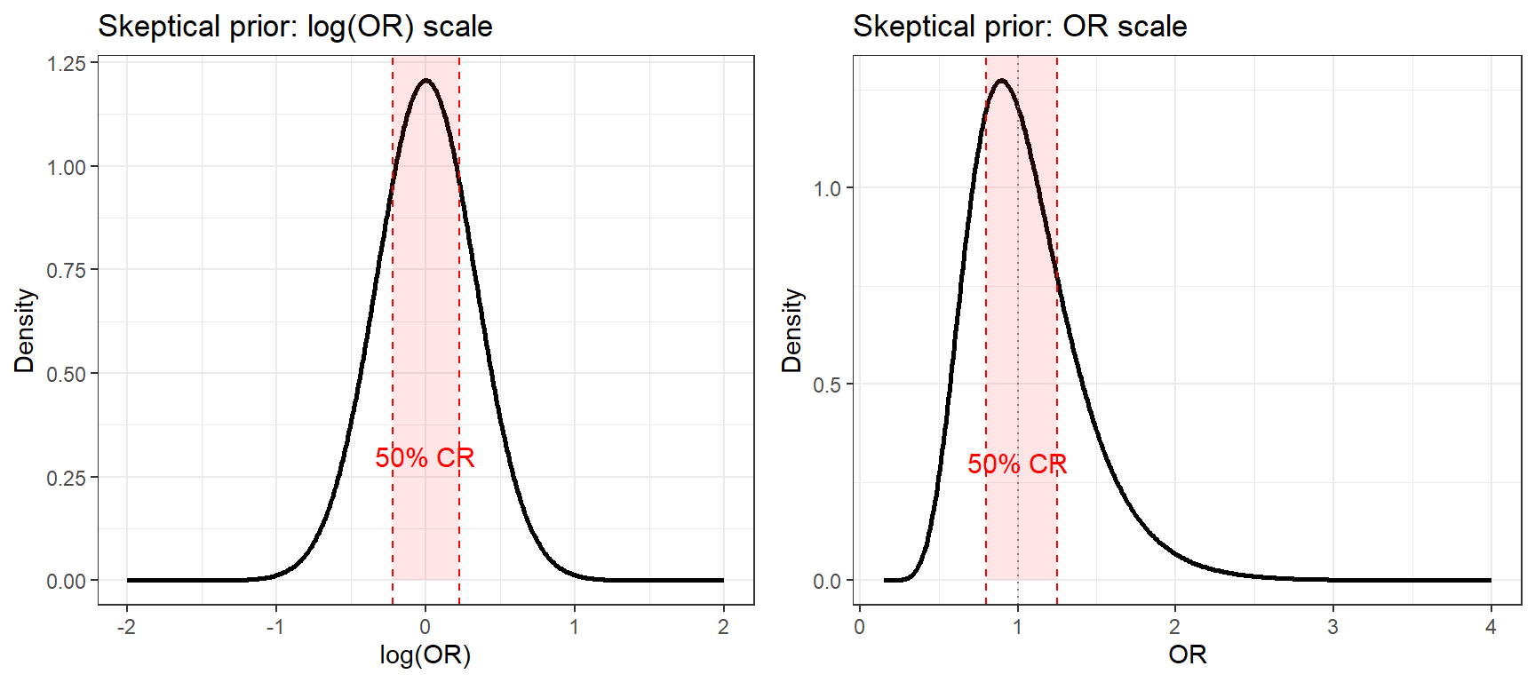

Key observations

On the log(OR) scale the prior is symmetric, the normal distribution is centered at 0 (OR = 1) and the 50% credible region (shaded) spans the similarity zone (0.8, 1.25).
On the OR scale the prior appears right-skewed. This is expected: OR is a log-normal quantity, so even a symmetric prior on log(OR) looks asymmetric on the natural scale.
A 50% prior probability within the similarity region is a moderately skeptical choice. Making it narrower (e.g., 75% within the same region) would express stronger skepticism.