require(tidyverse)
library(brms)
library(bayesplot)
library(DT)
library(gtsummary)
library(knitr)Tutorial 5
Hands-on exercise fitting regression models
1. How scientific are various disciplines
1.1 Study background
These data are collected from a survey study. Doctors across Canada were asked in a survey how many hours per week they spent on scientific research.
dat <- read.table("data/HowScientific.txt",header = T)

dat %>% datatable(
  rownames = FALSE,
  options = list(
 pageLength = 35,
    columnDefs = list(list(className = 'dt-center',
                      targets = 0:3))))
We can easily rank the disciplines from highest to lowest based on the observed means:
dat <- dat[order(dat$Hours,decreasing = F),]
dat$Specialty <- factor(dat$Specialty,
                      levels=dat$Specialty)
dat %>% ggplot(aes(y=Specialty,x=Hours))+
  geom_point()+
  geom_errorbar(aes(xmin=Hours-SD, xmax=Hours+SD), width=.2, colour = "red", position=position_dodge(0.05))+
  labs(title = paste("Research hour by specialty", "(Mean hours +/- SD)", sep = " "))+
  theme_bw()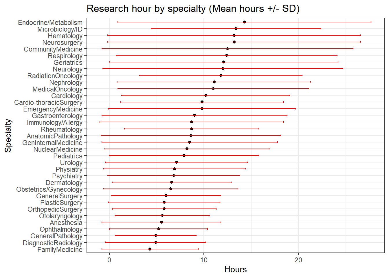
1.2 Modelling ranking and data uncertainty
How sure are we of these rankings - there is uncertainty about the true value of the mean in each group - we know the group mean - although we do not have all the data in each group, we have the SD and n (this resembles a meta analysis!)
Objective of this analysis is to quantify the probability that a particular discipline is ``more scientific’’ than another discipline.
1.3 Model building
- We can specify a model for each discipline, index by i.
- The observed mean hours are sampled from a normal distribution with an unknown mean \(\mu_i\) and and known variance of the mean. Under the central limit theorem, the variance of mean is
\[var(\mu) = SE(\mu)^2 = SD^2/n\]
- Thus, we have the following model/likelihood.
\[ Hours_i \sim N(\mu_i, sd^2_{i}/n_i)) \]
- We will put a random effects prior on the mu_i. Can you see that \(\mu_0\) and \(\sigma^2\) as two hyper priors
\[ \mu_i \sim N(\mu_0, \sigma^2) \]
We are interest in estimating the values of \(\mu_i\) as these are the true unknown mean hours for each specialty, which we want to compare (rather than the observed hours).
This can be easily done in brms. The function has notation that allows us to supply a known SD.
1.4 Fitting a random intercept model (partical pooling)
We can fit a random intercept model, here we assume there is a common underlying research hours but there exists random variation across disciplines.
We can use the brms default priors.
dat$SE_mean <- dat$SD/sqrt(dat$n)
fit1 <- brm(data = dat,
            family = gaussian,
            Hours | se(SE_mean) ~ 1 + (1 | Specialty),
            iter = 5000,
            warmup = 4000,
            cores = 4,
            chains = 4,
            seed = 15)
# saveRDS(fit1, "data/tut4_fit1")
fit1 <- readRDS("data/tut4_fit1")
prior_summary(fit1) prior class coef group resp dpar nlpar lb ub
student_t(3, 8.6, 3.9) Intercept
student_t(3, 0, 3.9) sd 0
student_t(3, 0, 3.9) sd Specialty 0
student_t(3, 0, 3.9) sd Intercept Specialty 0
source
default
default
(vectorized)
(vectorized)print(fit1) Family: gaussian
Links: mu = identity; sigma = identity
Formula: Hours | se(SE_mean) ~ 1 + (1 | Specialty)
Data: dat (Number of observations: 35)
Draws: 4 chains, each with iter = 5000; warmup = 4000; thin = 1;
total post-warmup draws = 4000
Group-Level Effects:
~Specialty (Number of levels: 35)
Estimate Est.Error l-95% CI u-95% CI Rhat Bulk_ESS Tail_ESS
sd(Intercept) 2.84 0.37 2.20 3.65 1.01 418 1093
Population-Level Effects:
Estimate Est.Error l-95% CI u-95% CI Rhat Bulk_ESS Tail_ESS
Intercept 8.65 0.49 7.66 9.60 1.01 354 543
Family Specific Parameters:
Estimate Est.Error l-95% CI u-95% CI Rhat Bulk_ESS Tail_ESS
sigma 0.00 0.00 0.00 0.00 NA NA NA
Draws were sampled using sampling(NUTS). For each parameter, Bulk_ESS
and Tail_ESS are effective sample size measures, and Rhat is the potential
scale reduction factor on split chains (at convergence, Rhat = 1).The estimated mean research hours across discipline is 8.65 (7.66, 9.60).
There is substantial between specialty variation estimated at 2.84 (2.20, 3.65).
We can produce Bayesian model estimated research hours by discipline and rank them!
x <- posterior_samples(fit1)
names(x)
[1] "b_Intercept"
[2] "sd_Specialty__Intercept"
[3] "sigma"
[4] "r_Specialty[FamilyMedicine,Intercept]"
[5] "r_Specialty[DiagnosticRadiology,Intercept]"
[6] "r_Specialty[GeneralPathology,Intercept]"
[7] "r_Specialty[Ophthalmology,Intercept]"
[8] "r_Specialty[Anesthesia,Intercept]"
[9] "r_Specialty[Otolaryngology,Intercept]"
[10] "r_Specialty[OrthopedicSurgery,Intercept]"
[11] "r_Specialty[PlasticSurgery,Intercept]"
[12] "r_Specialty[GeneralSurgery,Intercept]"
[13] "r_Specialty[Obstetrics/Gynecology,Intercept]"
[14] "r_Specialty[Dermatology,Intercept]"
[15] "r_Specialty[Psychiatry,Intercept]"
[16] "r_Specialty[Physiatry,Intercept]"
[17] "r_Specialty[Urology,Intercept]"
[18] "r_Specialty[Pediatrics,Intercept]"
[19] "r_Specialty[NuclearMedicine,Intercept]"
[20] "r_Specialty[GenInternalMedicine,Intercept]"
[21] "r_Specialty[AnatomicPathology,Intercept]"
[22] "r_Specialty[Rheumatology,Intercept]"
[23] "r_Specialty[Immunology/Allergy,Intercept]"
[24] "r_Specialty[Gastroenterology,Intercept]"
[25] "r_Specialty[EmergencyMedicine,Intercept]"
[26] "r_Specialty[Cardio-thoracicSurgery,Intercept]"
[27] "r_Specialty[Cardiology,Intercept]"
[28] "r_Specialty[MedicalOncology,Intercept]"
[29] "r_Specialty[Nephrology,Intercept]"
[30] "r_Specialty[RadiationOncology,Intercept]"
[31] "r_Specialty[Neurology,Intercept]"
[32] "r_Specialty[Geriatrics,Intercept]"
[33] "r_Specialty[Respirology,Intercept]"
[34] "r_Specialty[CommunityMedicine,Intercept]"
[35] "r_Specialty[Neurosurgery,Intercept]"
[36] "r_Specialty[Hematology,Intercept]"
[37] "r_Specialty[Microbiology/ID,Intercept]"
[38] "r_Specialty[Endocrine/Metabolism,Intercept]"
[39] "lprior"
[40] "lp__" names(x) <- gsub("r_Specialty","",names(x))
names(x) <- gsub(",Intercept","",names(x))
# x <- x %>% mutate(across(c(-sd_Specialty__Intercept,-sigma)))
x <- x[,-c(2,3,39,40)] #remove sd and likelihood estimates;
x <- x[,-1] + x[,1] #remove the overall mean estimate and add that value to each remaining columns to obtain specialty specific hours;
x %>% datatable(
rownames = FALSE,
options = list(
columnDefs = list(list(className = 'dt-center', targets = 5)),
pageLength = 10))- Now creating table to show posterior summary of the estimated hours by specialty
ranks <- apply(x, MARGIN = 1, FUN = rank)
qranks <- round(apply(ranks, MARGIN = 1, FUN = quantile, c(0.5, 0.025, 0.975)),0)
kable(t(qranks))| 50% | 2.5% | 97.5% | |
|---|---|---|---|
| [FamilyMedicine] | 1 | 1 | 2 |
| [DiagnosticRadiology] | 3 | 2 | 5 |
| [GeneralPathology] | 3 | 1 | 7 |
| [Ophthalmology] | 4 | 2 | 7 |
| [Anesthesia] | 5 | 3 | 8 |
| [Otolaryngology] | 6 | 3 | 10 |
| [OrthopedicSurgery] | 7 | 4 | 10 |
| [PlasticSurgery] | 8 | 3 | 12 |
| [GeneralSurgery] | 8 | 5 | 11 |
| [Obstetrics/Gynecology] | 11 | 8 | 14 |
| [Dermatology] | 11 | 7 | 15 |
| [Psychiatry] | 12 | 10 | 14 |
| [Physiatry] | 13 | 8 | 17 |
| [Urology] | 14 | 8 | 18 |
| [Pediatrics] | 16 | 14 | 19 |
| [NuclearMedicine] | 17 | 10 | 24 |
| [GenInternalMedicine] | 18 | 15 | 21 |
| [AnatomicPathology] | 19 | 14 | 23 |
| [Rheumatology] | 19 | 14 | 24 |
| [Immunology/Allergy] | 19 | 9 | 28 |
| [Gastroenterology] | 20 | 15 | 25 |
| [EmergencyMedicine] | 23 | 18 | 28 |
| [Cardio-thoracicSurgery] | 22 | 16 | 28 |
| [Cardiology] | 24 | 20 | 28 |
| [MedicalOncology] | 26 | 20 | 33 |
| [Nephrology] | 26 | 20 | 33 |
| [RadiationOncology] | 29 | 23 | 34 |
| [Neurology] | 30 | 24 | 34 |
| [Geriatrics] | 29 | 21 | 35 |
| [Respirology] | 31 | 25 | 35 |
| [CommunityMedicine] | 30 | 24 | 35 |
| [Neurosurgery] | 30 | 21 | 35 |
| [Hematology] | 31 | 22 | 35 |
| [Microbiology/ID] | 33 | 28 | 35 |
| [Endocrine/Metabolism] | 34 | 27 | 35 |
- For any pair of specialties, we can calculate the probability that one is more scientific than another
mean(x[,"[Microbiology/ID]"] < x[,"[Endocrine/Metabolism]"])[1] 0.55675mean(x[,"[Nephrology]"] < x[,"[Endocrine/Metabolism]"])[1] 0.9425