require(tidyverse)
library(brms)
library(bayesplot)
library(DT)
library(gtsummary)
library(knitr)
library(plotly)Tutorial 6
Exercise fitting a Poisson regression model
The data and analysis are taken from (Kalesan et al. 2016) and Prof. Brian Reich’s lecture notes.
The objective is to study the association of different firearm laws with overall firearm mortality, homicide firearm mortality, and suicide firearm mortality across all US states.
- The response for state \(i\) is the number of gun related homicides in 2010.
- \(N_i\) is the state population in 2010.
- Main exposure of interest is the number of state gun laws, denote as \(X_i\).
- There are five other covariates (\(Z\))
- 2009 firearm death rate per 10,000 people
- Firearm ownership rate quartile
- Unemployment rate quartile
- Non-firearm homicide rate quartile
- Firearm export rate quartile
We will analyze these data using the Bayesian Poisson regression model \[Y_i \sim \mbox{Poisson}(N_i\lambda_i) \mbox{ and } \mbox{log}(\lambda_i)= \gamma + \sum_{j=1}^5Z_{ij}\alpha_j + X_i\beta,\]
where \(\alpha_0,...,\alpha_5,\beta\) are the unknown regression coefficients.
dat <- read.table("data/US_homicide.txt",header = T)

dat %>% datatable(
  rownames = FALSE,
  options = list(
 pageLength = 50,
    columnDefs = list(list(className = 'dt-center',
targets = 0:8))))- Creating interactive maps in R using plotly.
plot_ly(
  type = "choropleth",
  locations = dat$state_code,
  locationmode = "USA-states",
  z = dat$gun_laws,
  colors = "Blues"
) %>%
  layout(geo = list(scope = "usa"),
title = 'Number of Gun Laws per state')plot_ly(
type = "choropleth",
locations = dat$state_code,
locationmode = "USA-states",
z = dat$homicide_2010,
colors = "YlOrRd"
) %>%
layout(geo = list(scope = "usa"),
title = 'Number of Homicide in 2010')Perform Poisson regression using MLE
mle <- glm(homicide_2010~gun_laws+X2009.rate+
               Firearm.ownership.rate.quartile+
               Unemployment.rate.quartile+
               Non.firearm.homicide.rate.quartile+
               Firearm.export.rate.quartile,data = dat, family="poisson")
summary(mle)
Call:
glm(formula = homicide_2010 ~ gun_laws + X2009.rate + Firearm.ownership.rate.quartile +
    Unemployment.rate.quartile + Non.firearm.homicide.rate.quartile +
    Firearm.export.rate.quartile, family = "poisson", data = dat)

Coefficients:
                                    Estimate Std. Error z value Pr(>|z|)
(Intercept)                         5.310547   0.031649 167.796  < 2e-16 ***
gun_laws                            0.006513   0.001442   4.517 6.26e-06 ***
X2009.rate                          0.846766   0.034454  24.576  < 2e-16 ***
Firearm.ownership.rate.quartile    -0.019885   0.007965  -2.497   0.0125 *
Unemployment.rate.quartile          0.178849   0.006142  29.118  < 2e-16 ***
Non.firearm.homicide.rate.quartile  0.351802   0.007942  44.297  < 2e-16 ***
Firearm.export.rate.quartile       -0.524407   0.007187 -72.967  < 2e-16 ***
---
Signif. codes:  0 '***' 0.001 '**' 0.01 '*' 0.05 '.' 0.1 ' ' 1

(Dispersion parameter for poisson family taken to be 1)

    Null deviance: 25001  on 49  degrees of freedom
Residual deviance: 12786  on 43  degrees of freedom
AIC: 13191

Number of Fisher Scoring iterations: 5
Bayesian regression model using brms
model1 <- brm(homicide_2010~gun_laws+X2009.rate+
               Firearm.ownership.rate.quartile+
               Unemployment.rate.quartile+
               Non.firearm.homicide.rate.quartile+
               Firearm.export.rate.quartile,
    data = dat,
    family = "poisson",
    sample_prior=T,
    prior = c(prior(normal(0, 100), class = "Intercept"),
              prior(normal(0, 10), class = "b")),
    chains = 4,
    iter = 7500,
    warmup = 5000,
    cores = 4,
    seed = 123,
    silent = 2,
    refresh = 0)

saveRDS(model1, "data/tut5_poisson_1")- Posterior summary
model1 <- readRDS("data/tut5_poisson_1")
plot(model1)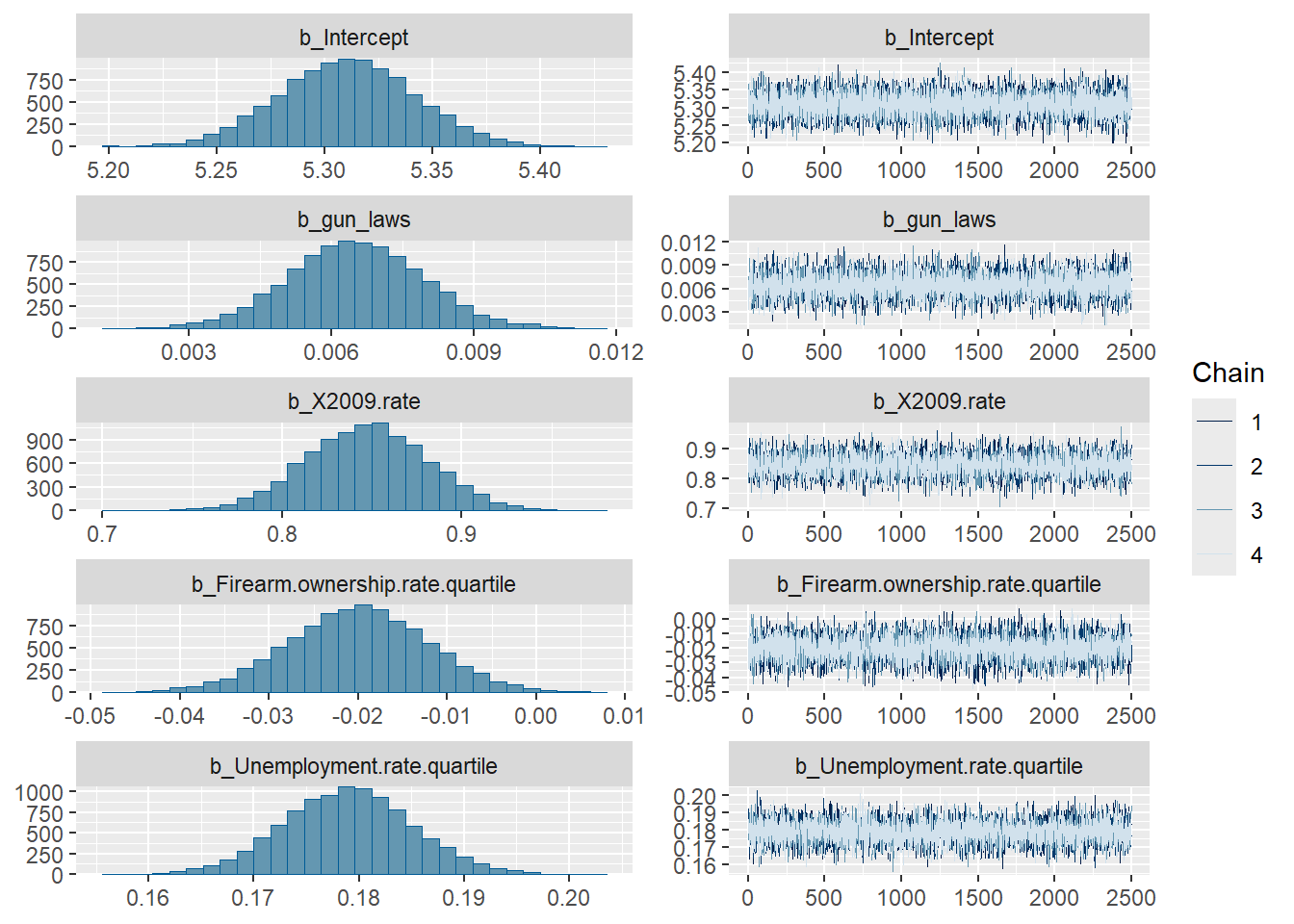
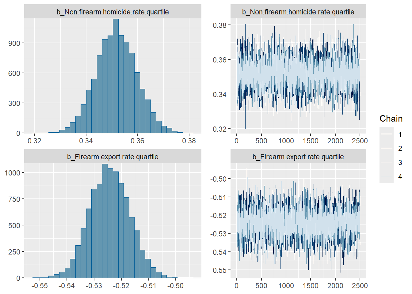
print(model1) Family: poisson
Links: mu = log
Formula: homicide_2010 ~ gun_laws + X2009.rate + Firearm.ownership.rate.quartile + Unemployment.rate.quartile + Non.firearm.homicide.rate.quartile + Firearm.export.rate.quartile
Data: dat (Number of observations: 50)
Draws: 4 chains, each with iter = 7500; warmup = 5000; thin = 1;
total post-warmup draws = 10000
Regression Coefficients:
Estimate Est.Error l-95% CI u-95% CI Rhat
Intercept 5.31 0.03 5.25 5.37 1.00
gun_laws 0.01 0.00 0.00 0.01 1.00
X2009.rate 0.85 0.03 0.78 0.91 1.00
Firearm.ownership.rate.quartile -0.02 0.01 -0.04 -0.00 1.00
Unemployment.rate.quartile 0.18 0.01 0.17 0.19 1.00
Non.firearm.homicide.rate.quartile 0.35 0.01 0.34 0.37 1.00
Firearm.export.rate.quartile -0.52 0.01 -0.54 -0.51 1.00
Bulk_ESS Tail_ESS
Intercept 11915 8652
gun_laws 9792 7757
X2009.rate 7445 6965
Firearm.ownership.rate.quartile 9853 6861
Unemployment.rate.quartile 9602 7195
Non.firearm.homicide.rate.quartile 8491 7129
Firearm.export.rate.quartile 9211 7616
Draws were sampled using sampling(NUTS). For each parameter, Bulk_ESS
and Tail_ESS are effective sample size measures, and Rhat is the potential
scale reduction factor on split chains (at convergence, Rhat = 1).- Comparing prior and posterior
s1 <- posterior_samples(model1)- We are interested in computing the posterior distributions of RR.
s1 <- posterior_samples(model1)
beta <- data.matrix(s1[,c("b_gun_laws",
                          "b_X2009.rate",
                          "b_Firearm.ownership.rate.quartile",
                          "b_Unemployment.rate.quartile",
                          "b_Non.firearm.homicide.rate.quartile",
                          "b_Firearm.export.rate.quartile")])

my.summary <- function(x){
  round(c(Mean=mean(x), Median=median(x), low=quantile(x,0.025), high=quantile(x, 0.975)),2)
}

t(apply(exp(beta),2,my.summary))
Mean Median low.2.5% high.97.5%
b_gun_laws 1.01 1.01 1.00 1.01
b_X2009.rate 2.33 2.33 2.18 2.49
b_Firearm.ownership.rate.quartile 0.98 0.98 0.96 1.00
b_Unemployment.rate.quartile 1.20 1.20 1.18 1.21
b_Non.firearm.homicide.rate.quartile 1.42 1.42 1.40 1.44
b_Firearm.export.rate.quartile 0.59 0.59 0.58 0.60- suppose we are interested in predicting homicide rates for each state
pp<-posterior_predict(model1)
mean.pp<- colMeans(pp)
lci.pp<- apply(pp, 2, function(x) quantile(x, 0.025))
uci.pp<- apply(pp, 2, function(x) quantile(x, 0.975))

pp.table <- data.frame(State = dat$state,
                       homicide_obs = dat$homicide_2010,
                       posterior_predict_homicide = round(mean.pp,0),
                       CI = paste0("(",round(lci.pp,0),",",round(uci.pp,0),")"))

pp.table %>%
  datatable(
  rownames = F,
  options = list(
 pageLength = 50,
    searching = FALSE,
    columnDefs = list(list(className = 'dt-center',
targets = 0:3))))dat$homicide_postpred <- round(mean.pp,0)
plot_ly(
type = "choropleth",
locations = dat$state_code,
locationmode = "USA-states",
z = dat$homicide_postpred,
colors = "YlOrRd"
) %>%
layout(geo = list(scope = "usa"),
title = 'Model predicted Number of Homicide in 2010')References
Kalesan, Bindu, Matthew E Mobily, Olivia Keiser, Jeffrey A Fagan, and Sandro Galea. 2016. “Firearm Legislation and Firearm Mortality in the USA: A Cross-Sectional, State-Level Study.” The Lancet 387 (10030): 1847–55.