Prior Distributions
Learning Objectives
- Learn different ways of selecting and constructing priors
1. Choosing the prior distribution
Incorporating prior information in statistical analysis is a unique feature for Bayesian modelling
1.1 Types of priors
Generally speaking, there are two types of priors: subjective priors and objective priors.
- Subjective priors
- based on historical data
- Characterization of personal/expert opinion
- Selection of “standard” (clinical) prior distributions
- use sparsity promoting prior (i.e., shrinkage prior) to reduce the number of parameters to be estimated to improve estimation efficiency and avoid over-fitting
- objective priors
- priors that don’t bring subjective information into the analysis
- reference priors, vague priors (e.g., flat priors, Jeffreys’ priors)
- weakly informative priors
1.2 Prior Elicitation
- Expert knowledge is a valuable source of information
- Prior elicitation is a key tool for summarizing and translating expert knowledge into a quantitative probability distribution
- Expert elicited priors can be used in the design and analysis the study.
when should we use prior elicitation?
From (Lesaffre, Baio, and Boulanger 2020)
- Factors favouring elicitation
- (no information) Inadequate empirical data are available to inform a decision (no information)
- (conflicting information) Multiple sources of empirical data are available of differing levels of relevance
- (no consensus) Lack of scientific consensus, or when reliable evidence or legitimate models are in conflict, with a need to quantify the uncertainty due to disagreement
- (when you can!) Appropriate experts (and financial resources) are available and elicitation can be completed within the required time frame
- Factors not favouring elicitation
- (not useful) A large body of empirical data (of suitable quality and relevance) exists with a high degree of consensus
- (not important) The information that an expert elicitation could provide is not critical to the assessment or decision
- (too much effort) Available expertise and/or financial resources are insufficient to conduct a robust and defensible elicitation
Methods for prior elicitation
- Fixed and variable interval methods
- expert is asked to consider a fixed value or a plausible range for the parameter
- e.g., “what is the probability that a healthy 30 year-old non-healthcare worker in Ontario will have received a COVID-19 vaccine by September 1 2021?”
- e.g., “Based on your expertise and experience, please choose the LOWER and UPPER plausible values for the number of patients who would end up being admitted to hospital out of 100 similar patients with the presented case of bronchiolitis”
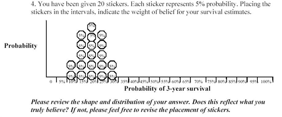
- Roulette or Chips in Bins
- expert is given a “chip” and asked to place it to a distribution
- proportion of chips allocated to a particular bin priors the expert’s knowledge on the true value of the parameter (that it lies in that bin)
- generally accepted as an intuitive elicitation methods for experts
Aggregating expert judgement
There are two general approaches to summarizing the estimates from the experts.
- Aggregate the distributions
- combine these multiple distribution using mathematical aggregation, also called “pooling”
- Elicit a distribution from each expert separately and “all opinions are considered”
- easier elicitation process and minimal interaction between experts
- when individual priors are very diverse, mathematical pooling may create an average set of judgments that lacks any substantive meaning
- Aggregate the experts
- gather expert belief and elicit a single distribution, also called behavioural aggregation.
- can help to provide insights and resolve differences of opinion
- minority or extreme opinions may be lost in building a common group view
- requires a trained facilitator to manage the elicitation process and the interactions between the experts to ensure that the process is not dominated by only one or two experts
Three protocols
- Most popular. Sheffield Elicitation Framework (SHELF). The SHELF protocol is a behavioral aggregation method that uses two rounds of judgments. (O’Hagan et al. 2006)
- In the first round, individuals make private judgement
- In the second round, those judgments are reviewed before the group agrees on consensus judgement.
- Delphi Method. The Delphi is similar to SHELF as it is a behavioral aggregation method with two or more rounds except that anonymity is maintained in terms of who gave which answers.
- unlike SHELF, experts provide their judgments individually with no interaction and a pooling rule is required across expert final distributions.
Evaluating prior elicitation
Reference: Methods to elicit beliefs for Bayesian priors: a systematic review (2010), by johnson et al. (Johnson, Tomlinson, Hawker, Granton, and Feldman 2010).
- Reviewed prior elicitation on validity, reliability, responsiveness, and feasibility
Example expert elicitation from (Johnson, Tomlinson, Hawker, Granton, Grosbein, et al. 2010)
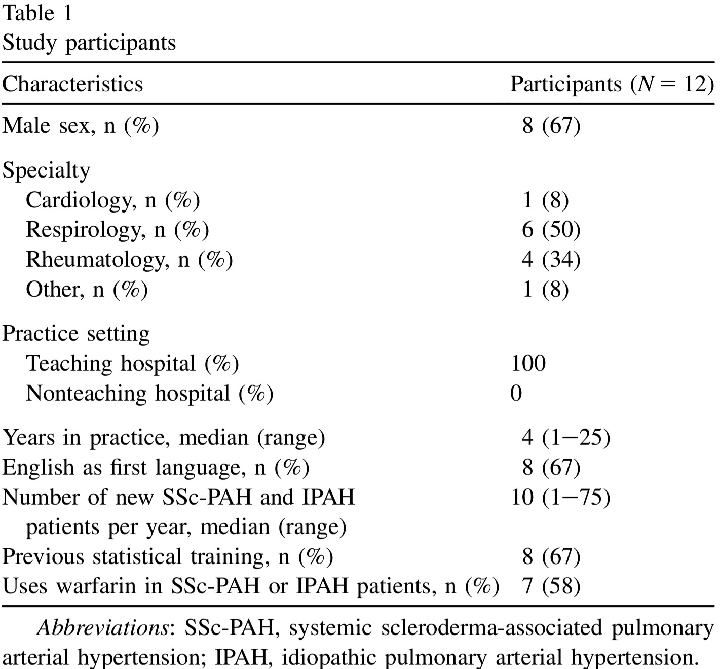
1. Participants
- single centre 12 academic specialists at the University of Toronto who treat systemic sclerosis (scleroderma)-associated pulmonary arterial hypertension (SSc-PAH) and idiopathic pulmonary arterial hypertension (IPAH) patients were recruited (single centre)
2. Procedure
A face-to-face interview was conducted with each participant using a standardized script
Conducted a sample questionnaire (pre-run) on unrelated clinical example to introduce the questions and process to participants.
Design and deliver questionnaires for elicitation (focus on clarity)
- “Question 1. For an average group of newly diagnosed scleroderma patients with pulmonary arterial hypertension treated with the standard of care at your institution but not treated with warfarin, what do you believe is the probability of being alive at 3 years? Please indicate your answer by putting an X on the line.”
- “Question 3. There may be some uncertainty around your estimate of survival. You may believe that the probability of survival could be a little lower or a little higher. Please indicate the lower boundary of your estimate for which you believe there is very little probability that the true estimate could be less than. Please indicate the higher boundary of your estimate for which you believe there is very little probability that the true estimate could be greater than. You have indicated that the lower boundary is X% and the upper boundary is Y%.”
Assess measurement properties
- face Validity
- e.g., do you feel that this questionnaire evaluated your belief about the effect of warfarin on survival in idiopathic and/or SSc-PAH?
- convergent construct validity
- What overall effect do you believe warfarin has on 3-year survival? Improves survival, worsens survival or has no effect on survival. Comparing results from this question to the elicitated belief and see if they match!
- expected moderate to good agreement between the two questions categorizing the effect of warfarin on survival
- feasibility
- e.g., how long it takes to complete the questionnaire
- reliability
- Test reliability of the elicitation procedure was tested by administering the questionnaire to participants on two occasions 1-2 weeks apart.
- face Validity
3. Results
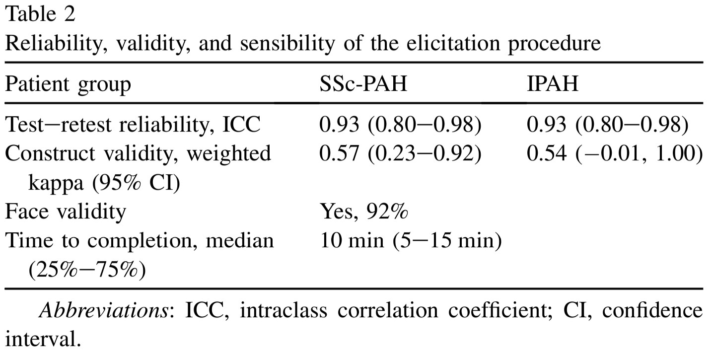
- Good validity, reliability, and feasibility
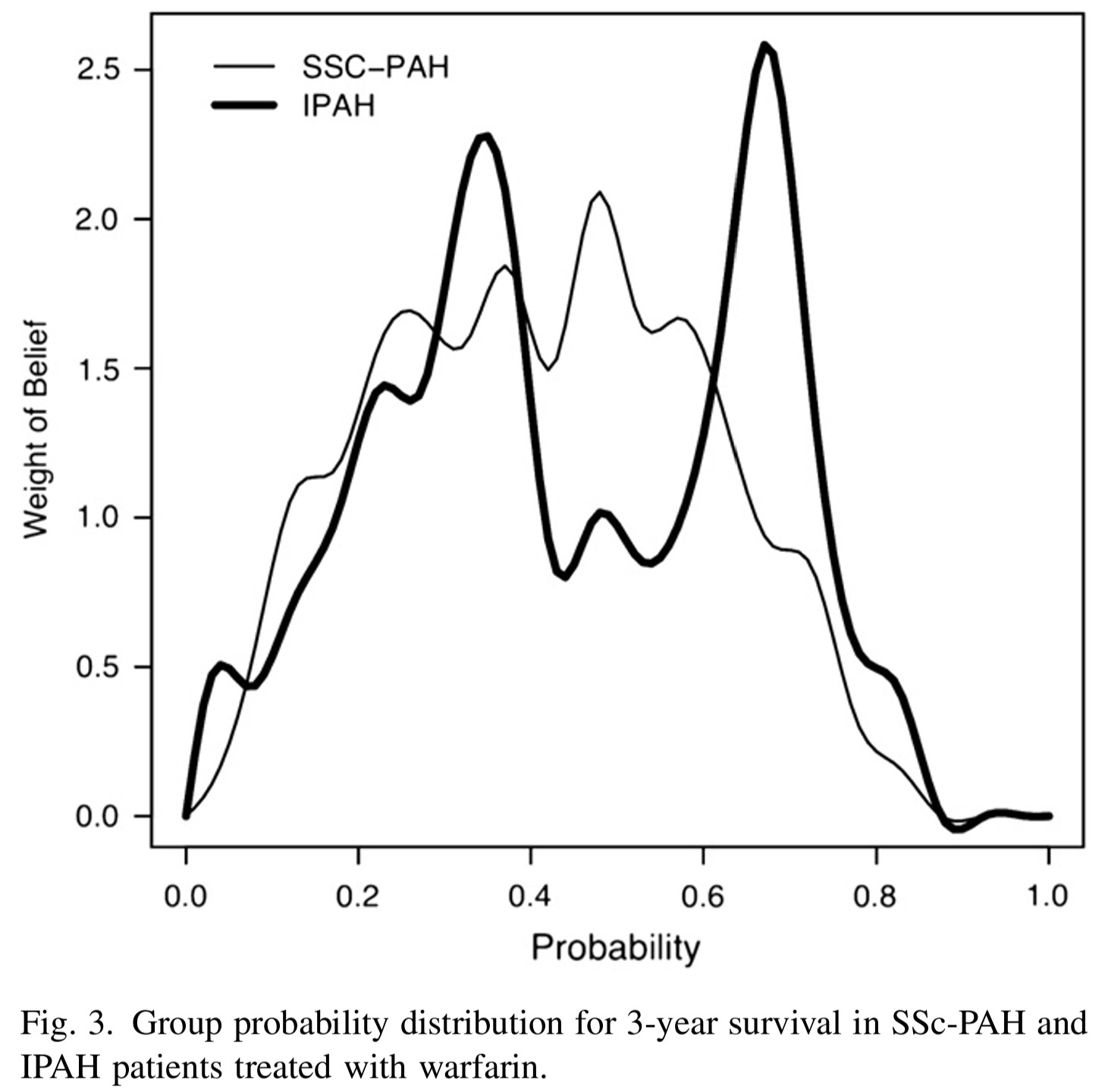
- The group probability distributions for SScPAH and IPAH patients treated with warfarin are wide.
- indicating variability in belief among experts
- The group probability distribution for SSc-PAH is unimodal and the group probability distribution for IPAH is bimodal.
- we can approximate these distributions using mixture distributions (see tutorial).
1.3 Default clinical priors
The following “default” clinical prior types are discussed in Section 5.5 of (David J. Spiegelhalter, Abrams, and Myles 2003) and further elaborated in (David J. Spiegelhalter 2004). They provide a principled vocabulary for expressing a range of prior beliefs, from skepticism to enthusiasm, in a transparent and prespecified way. Using these named prior types helps analysts communicate assumptions clearly and conduct meaningful sensitivity analyses.
“Non-informative” or “reference” priors
Non-informative (also called “reference”) priors attempt to let the data speak for themselves by placing minimal prior weight on any particular parameter value. As noted by (David J. Spiegelhalter 2004), such analyses have been proposed as a way of “making probability statements about parameters without being explicitly Bayesian.”
Key caveats:
- Non-informative priors are never truly “neutral”, they always encode some assumption, even if only implicitly.
- They can lead to inference problems in small samples or when events are rare, where the prior can have a surprisingly strong impact.
- The Stan development team maintains a Prior Choice Recommendations wiki with practical guidance on sensible default priors for common models.
Example 1: Non-informative prior on a proportion
Suppose you are estimating the 30-day mortality after elective non-cardiac surgery. Two common “off the shelf” non-informative priors for a binomial proportion \(\theta\) are:
- \(\theta \sim \text{Uniform}(0,1) \equiv \text{Beta}(1,1)\), assigns equal probability to all values of \(\theta\) between 0 and 1.
- Jeffreys prior: \(\theta \sim \text{Beta}(0.5, 0.5)\), a principled non-informative prior derived from Fisher information. It has the appealing property of being invariant to reparameterization (e.g., it remains non-informative whether you parameterize by \(\theta\) or \(\log(\theta/(1-\theta))\)). Posterior estimates under this prior closely resemble frequentist estimates.
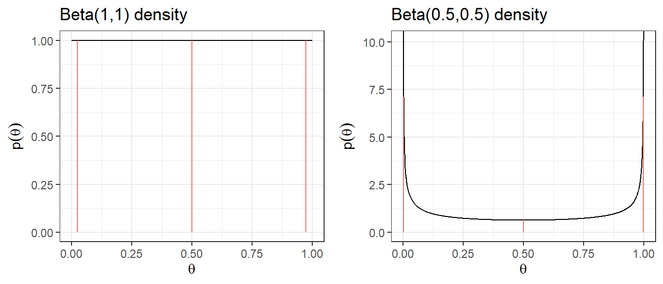
| Prior | median | q2.5 | q97.5 | Pr(\(\theta\)< 0.25) | Pr(\(\theta\)< 0.5) | Pr(\(\theta\)< 0.75) |
|---|---|---|---|---|---|---|
| Beta(1,1) | 0.5 | 0.025 | 0.975 | 0.25 | 0.5 | 0.75 |
| Beta(0.5,0.5) | 0.5 | 0.002 | 0.998 | 0.333 | 0.5 | 0.667 |
Example 2: Non-informative prior on log-relative risk
When modelling a relative risk (RR) in a clinical trial, inference is typically done on the log(RR) scale because the log-transformed estimate has an approximately normal sampling distribution.
A common “off the shelf” non-informative prior for log(RR) is a normal distribution centered at 0 (corresponding to RR = 1, i.e., no treatment effect) with a large variance:
\[\log(RR) = \theta \sim N(0, \sigma^2 = 10^2)\]
- Prior 95% credible interval for log(RR): \(-19.6\) to \(19.6\)
- Prior 95% credible interval for RR: \(3 \times 10^{-9}\) to \(3 \times 10^{9}\), clearly implausible values!
A more sensible default choice for log-scale parameters (OR, RR, HR) is \(N(0, 5^2)\), which still allows a very wide range but avoids placing weight on extreme values that are clinically nonsensical. The table below compares several choices.
Code
plot.norm <- function(mu, sd){
  d <- tibble(mu.plot=seq(-25,25, by=0.01),
              density=dnorm(mu.plot, mu,sd))
  p <- ggplot(data=d, aes(mu.plot, density))+
      geom_line(col="black")+
      geom_segment(aes(x = qnorm(0.025,mu,sd),
                       y = 0,
                       xend = qnorm(0.025,mu,sd),
                       yend = dnorm(qnorm(0.025,mu,sd), mu,sd),colour = "segment"))+
      geom_segment(aes(x = qnorm(0.5,mu,sd),
                       y = 0,
                       xend = qnorm(0.5,mu,sd),
                       yend = dnorm(qnorm(0.5,mu,sd), mu,sd),colour = "segment"))+
      geom_segment(aes(x = qnorm(0.975,mu,sd),
                       y = 0,
                       xend = qnorm(0.975,mu,sd),
                       yend = dnorm(qnorm(0.975,mu,sd), mu,sd),colour = "segment"))+
      xlab(expression(mu))+
      ylab(expression(p(mu)))+
        ggtitle(paste0("N(",mu,",",sd^2,") density"))+
      expand_limits(y=c(0,0.15))+
      theme_bw()
p

}

ggarrange(plot.norm(0,10),
          plot.norm(0,5),
          plot.norm(0,4),
          plot.norm(0,3),
          nrow = 2,ncol=2, legend = "none")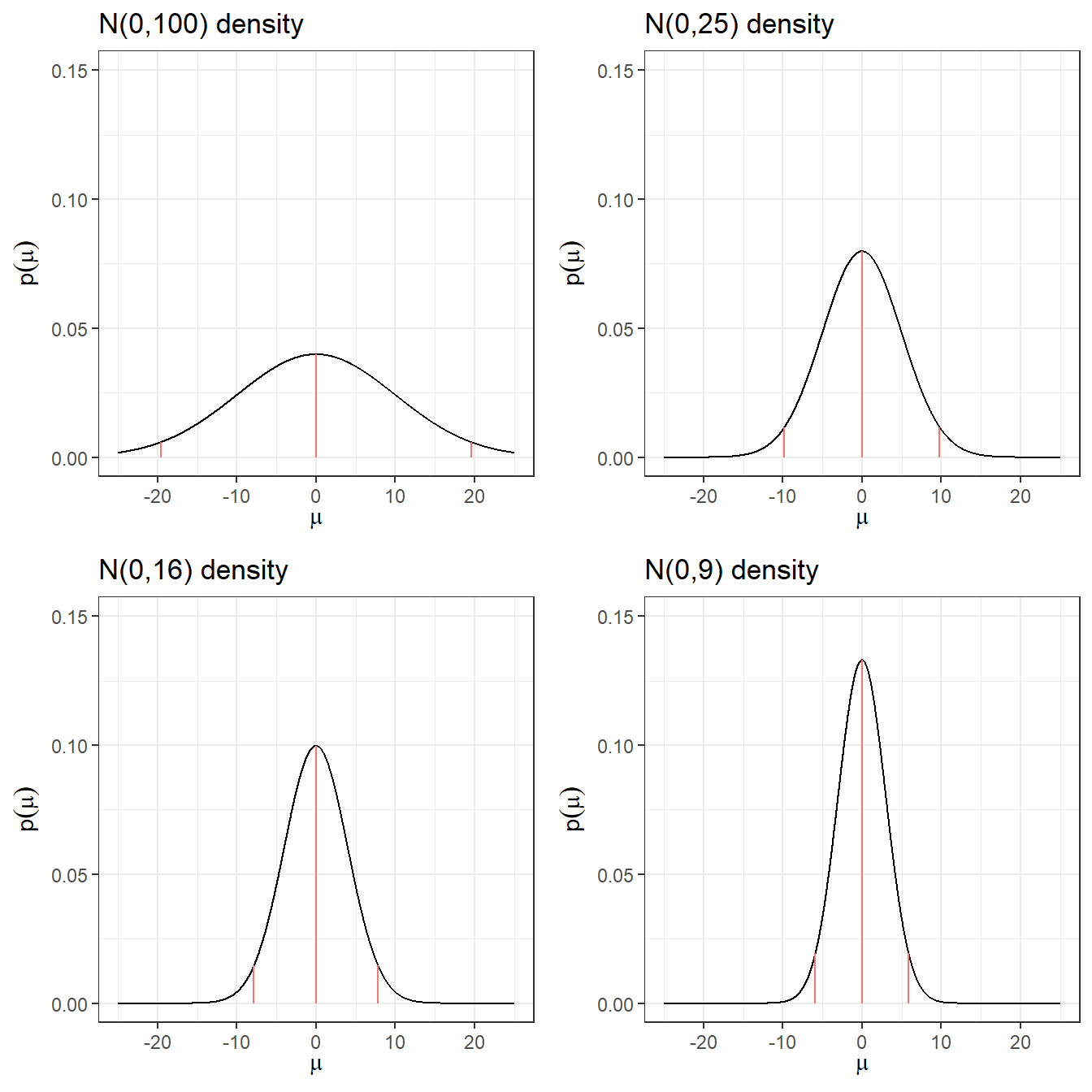
Code
res <- c("N(0,100)",
         round(qnorm(c(0.5, 0.025, 0.975), 0, 10),3),
         round(exp(qnorm(0.025, 0, 10)),10),
         round(exp(qnorm(0.975, 0, 10)),2))

res <- rbind(res, c("N(0,25)",
                  round(qnorm(c(0.5, 0.025, 0.975), 0, 5),3),
                  round(exp(qnorm(0.025, 0, 5)),10),
                  round(exp(qnorm(0.975, 0, 5)),2))
             )

res <- rbind(res, c("N(0,16)",
                  round(qnorm(c(0.5, 0.025, 0.975), 0, 4),3),
                  round(exp(qnorm(0.025, 0, 4)),10),
                  round(exp(qnorm(0.975, 0, 4)),2))
             )

res <- rbind(res, c("N(0,9)",
                  round(qnorm(c(0.5, 0.025, 0.975), 0, 3),3),
                  round(exp(qnorm(0.025, 0, 3)),10),
                  round(exp(qnorm(0.975, 0, 3)),2))
             )

res <- rbind(res, c("N(0,4)",
                  round(qnorm(c(0.5, 0.025, 0.975), 0, 2),3),
                  round(exp(qnorm(0.025, 0, 2)),10),
                  round(exp(qnorm(0.975, 0, 2)),2))
             )

res <- rbind(res, c("N(0,1)",
                  round(qnorm(c(0.5, 0.025, 0.975), 0, 1),3),
                  round(exp(qnorm(0.025, 0, 1)),10),
                  round(exp(qnorm(0.975, 0, 1)),2))
             )

knitr::kable(res, row.names = F,
col.names = c("Prior log(RR)","median log(RR)","q2.5 log(RR)","q97.5 log(RR)","q2.5 RR","q97.5 RR"))| Prior log(RR) | median log(RR) | q2.5 log(RR) | q97.5 log(RR) | q2.5 RR | q97.5 RR |
|---|---|---|---|---|---|
| N(0,100) | 0 | -19.6 | 19.6 | 0.0000000031 | 325098849.19 |
| N(0,25) | 0 | -9.8 | 9.8 | 0.0000554616 | 18030.5 |
| N(0,16) | 0 | -7.84 | 7.84 | 0.0003937258 | 2539.84 |
| N(0,9) | 0 | -5.88 | 5.88 | 0.0027950873 | 357.77 |
| N(0,4) | 0 | -3.92 | 3.92 | 0.019842524 | 50.4 |
| N(0,1) | 0 | -1.96 | 1.96 | 0.1408634941 | 7.1 |
Quick summary on non-informative priors
- The posterior can land on implausible values when there are few events in one or both groups, the prior is not protecting against this.
- These issues resolve somewhat with larger datasets, where a precise likelihood dominates the prior.
- With a large sample size or many events, even a vague prior is overwhelmed by the data and has minimal impact on the posterior.
Two key issues with “non-informative” priors
Issue 1: Uniform priors on one scale are not uniform on a transformed scale.
Suppose we set \(\theta \sim U(0,1)\) as a non-informative prior for the probability of an adverse event. However, once we transform \(\theta\) to the log-odds scale, \(\text{logit}(\theta) = \log\!\left(\frac{\theta}{1-\theta}\right)\), the distribution is far from uniform, it concentrates mass near \(-\infty\) and \(+\infty\). This means the prior is implicitly quite informative about extreme probabilities on the logit scale, even though it seemed neutral on the probability scale.
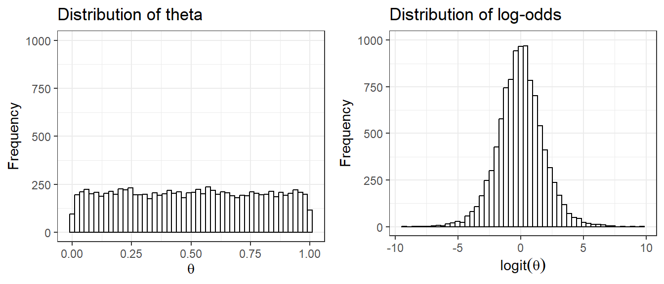
The Jeffreys prior \(\text{Beta}(0.5, 0.5)\) was specifically designed to avoid this issue, it is invariant to monotone transformations of the parameter.
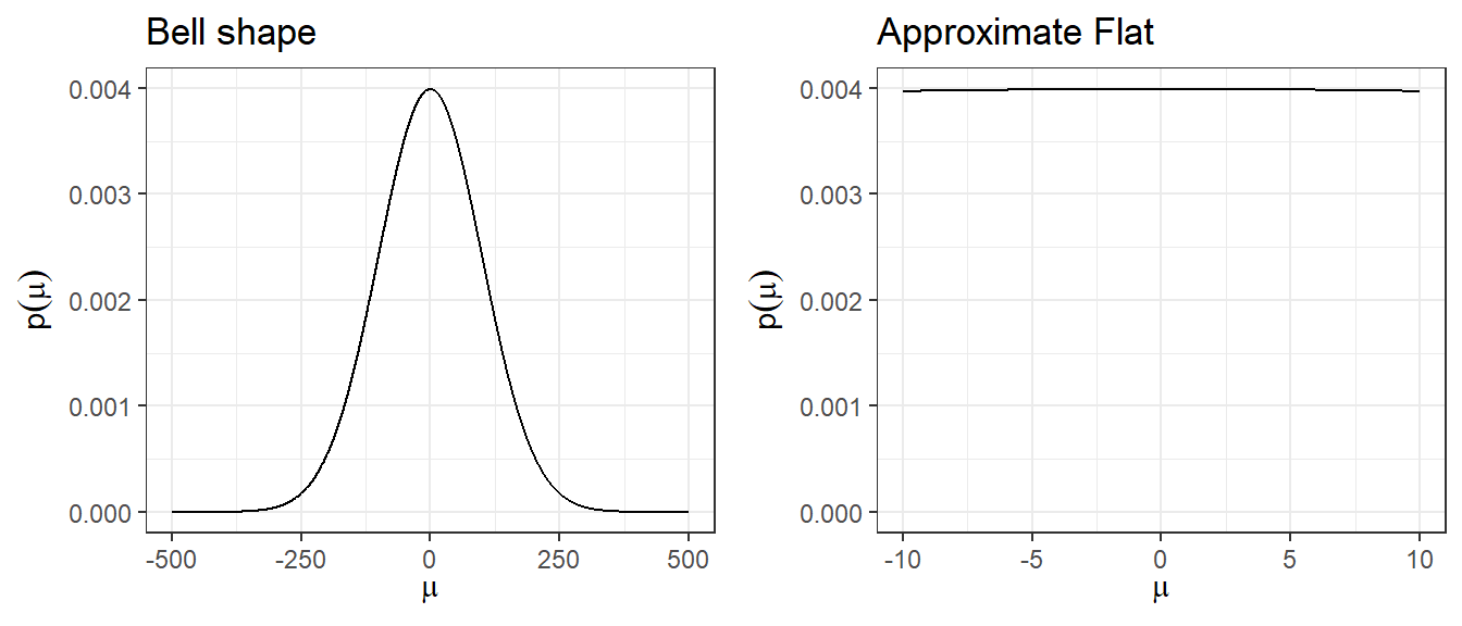
Issue 2: A large-variance normal prior is not truly flat, but is locally flat.
A prior like \(N(0, 100^2)\) has a bell shape and assigns higher density near 0 than at extreme values, so it is not uniformly non-informative. However, in the narrow region where the likelihood has support (i.e., where parameter values are plausible given the data), the normal density is approximately flat. This is the sense in which it is “locally non-informative.” For most practical purposes in clinical research, \(N(0, 5^2)\) achieves this local flatness while avoiding implausibly extreme values.
Minimally informative prior
A minimally informative prior occupies a middle ground between a non-informative prior and a strongly informative one. The goal is to use substantive clinical or scientific knowledge to rule out obviously implausible parameter values, without over-constraining inference (David J. Spiegelhalter, Abrams, and Myles 2003).
In practice, this means choosing a prior that places most of its mass on a plausible range of values, while still leaving tails wide enough to allow for surprise. Examples:
- For a RR for mortality in a trial, a prior that places most weight on values between 0.66 and 1.5 would be appropriate. A \(N(0,1)\) prior on log(RR) satisfies this. Tts 95% credible interval for RR spans roughly 0.14 to 7.1.
- For the between-person standard deviation of a 0-40 quality of life instrument, prior knowledge suggests values are unlikely to exceed 10. A \(\text{Gamma}(0.1, 0.1)\) prior on the precision (\(1/\sigma^2\)) is one possible choice.
The key principle: use domain knowledge to anchor the prior in a plausible region, but don’t mistake minimally informative for non-informative.
Skeptical prior
A skeptical prior expresses doubt that a treatment has a large beneficial effect (David J. Spiegelhalter, Abrams, and Myles 2003). This type of prior is appropriate when there is no strong prior evidence for efficacy and the analyst wants to require compelling data before concluding that a treatment works.
Formally, the skeptical prior:
- Is centred at the null (e.g., log(RR) = 0, corresponding to RR = 1, no effect).
- Has a spread chosen so that there is only a small prior probability (e.g., 5%) that the true effect is as large as the minimally clinically important difference (MCID).
The logic: if even a skeptic is convinced of effectiveness after seeing the data (i.e., the posterior still favour treatment), the evidence must be strong.
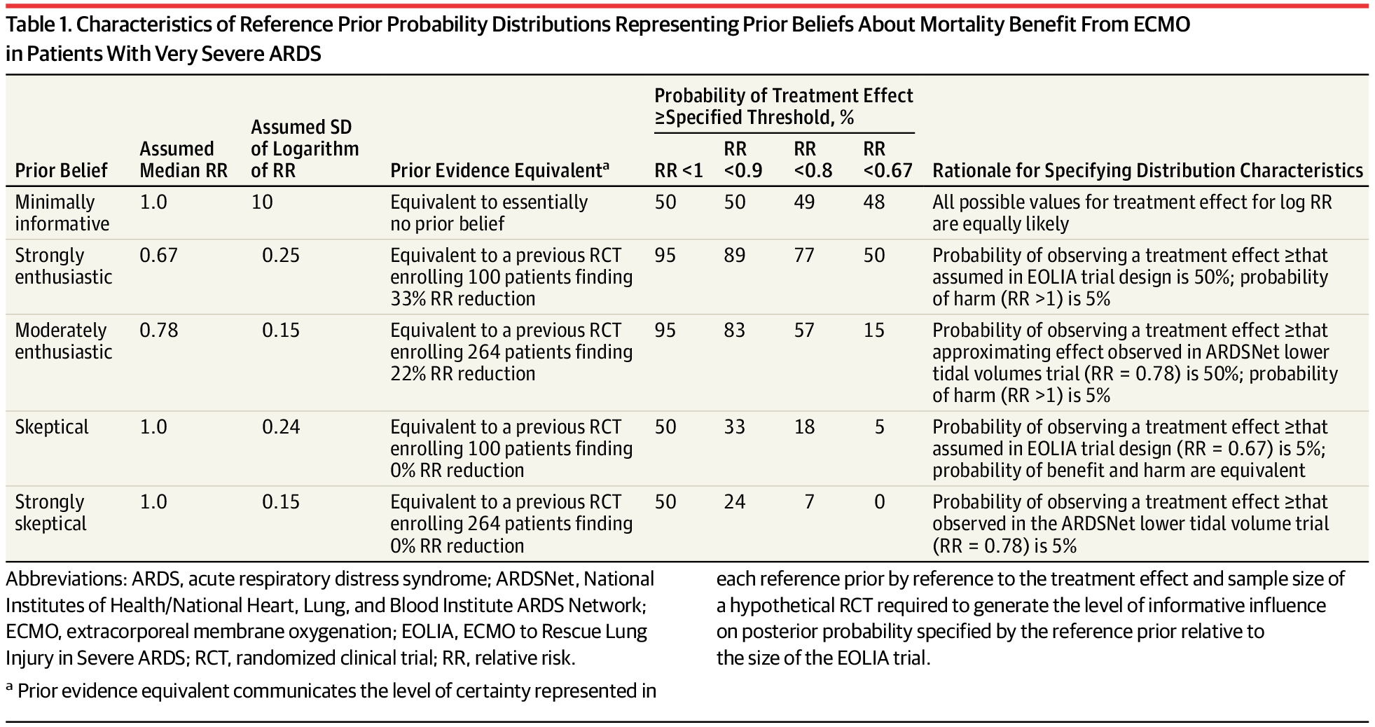
Skeptical prior specification: EOLIA trial example (Goligher et al. 2018)
Context: We want to assess the effect of ECMO vs. rescue lung-injury management on 60-day mortality in severe ARDS. Let \(\theta = \log(RR)\).
Step 1: Define the MCID. The MCID is an RR of 0.67 (a reduction from a 60% mortality rate to 40%), corresponding to \(\log(0.67) = -0.405\) on the log scale.
Step 2: Specify the skeptical prior mean. A skeptic sees no prior reason to expect benefit, so the mean is set at the null: \(\mu_0 = 0\) (i.e., RR = 1).
Step 3: Determine the prior SD so that only 5% prior probability lies below the MCID.
\[P\!\left(\log(RR) < -0.405\right) = P\!\left(Z < \frac{-0.405}{\sigma}\right) = 0.05\]
Since \(\Phi^{-1}(0.05) = -1.645\) (using qnorm(0.05, 0, 1)):
\[-1.645 \times \sigma = -0.405 \implies \sigma = \frac{0.405}{1.645} \approx 0.246\]
Result: The skeptical prior is \(\log(RR) \sim N(0,\; 0.246^2)\).
Optimistic/enthusiastic prior
An optimistic (enthusiastic) prior expresses belief that a treatment is likely to be effective, centered at the MCID rather than the null (David J. Spiegelhalter, Abrams, and Myles 2003). This type of prior is useful as a sensitivity analysis: if even an optimist cannot be convinced of efficacy after seeing the data, the evidence against effectiveness is very strong.
Formally, the optimistic prior:
- Is centered at the MCID (e.g., \(\log(\text{MCID})\) for a relative risk outcome).
- Has a spread chosen so that there is only a small prior probability (e.g., 5%) that the true effect is zero or harmful (i.e., RR \(\geq\) 1).
Optimistic prior specification: EOLIA trial example (Goligher et al. 2018)
Context: Same as above. \(\theta = \log(RR)\), MCID = 0.67, \(\log(0.67) = -0.405\).
Step 1: Set the prior mean at the MCID: \(\mu_0 = -0.405\).
Step 2: Determine the prior SD so that only 5% prior probability lies above the null (RR \(\geq\) 1, i.e., \(\log(RR) \geq 0\)).
\[P\!\left(\log(RR) > 0\right) = P\!\left(Z > \frac{0 - (-0.405)}{\sigma}\right) = 0.05\]
Since \(P(Z < 1.645) = 0.95\):
\[1.645 \times \sigma = 0.405 \implies \sigma = \frac{0.405}{1.645} \approx 0.246\]
Result: The enthusiastic prior is \(\log(RR) \sim N(-0.405,\; 0.246^2)\), or equivalently \(\log(RR) \sim N(\log(0.67),\; 0.246^2)\).
The table below (from Goligher et al. (2018)) summarizes all three prior types used in the EOLIA Bayesian reanalysis, making it easy to see how they differ in their assumptions:
Evaluating priors
After specifying a prior, it is good practice to assess whether it is well-calibrated, i.e., whether it is consistent with the observed data and with background knowledge. Two useful approaches are described in (David J. Spiegelhalter, Abrams, and Myles 2003):
1. Prior predictive check
The prior can be used to derive a prior predictive distribution for the data, that is, the distribution of outcomes you would expect to see before collecting data, averaged over the prior. Comparing this predictive distribution to the observed data provides a check on whether the prior is broadly consistent with the evidence.
Specifically, one can calculate the probability that a future observation would have a prior predictive ordinate at least as extreme as the one actually observed. When the predictive distribution is symmetric and unimodal, this is analogous to a two-sided p-value for testing prior-data compatibility. A very small value suggests the prior may be poorly calibrated.
2. Goodness-of-fit for elicited priors
When several candidate distributional forms are under consideration (e.g., normal, log-normal, beta), goodness-of-fit statistics, such as the Kolmogorov-Smirnov, can be used to evaluate which distribution best represents the elicited prior belief. The R package fitdistrplus provides convenient tools for this purpose.
1.4 Historical data
- Incorporating historical data in Bayesian analysis
- these can be formalized as a means of using past evidence as a basis for a prior distribution for a parameter of interest
- Meta-analysis is a very useful tool for evidence synthesis in clinical research
- We can directly use published meta-analysis results to construct priors
- if not available, one can also complete a meta-analysis to synthesis evidence for prior construction
- These types of prior are called data-derived priors.
- For example, in the Bayesian reanalysis of the EOLIA trial, data-derived priors are constructed from a Bayesian meta-analysis of published relevant studies.
- The posterior distribution (updated belief) of treatment effect is produced by combining data-derived prior with data from the current study.
Downweighting:
To reflect concerns about possible differences between the current and previous studies, the variance of the past studies can be inflated to receive less weight in the analysis on the pooled estimate of effect.
Data-derived prior from the Bayesian reanalysis of the EOLIA trial(Goligher et al. 2018)
- Data-derived prior was developed based on three relevant studies from a meta-analysis of ECMO for ARDS (Munshi et al. 2014)
- Three studies are (Peek et al. 2009), (Pham et al. 2013), and (Noah et al. 2011)
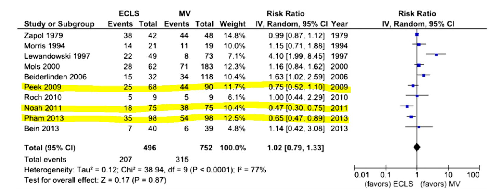
- After fitting a random effect model, the pooled RR is estimated as 0.64 with 95% CI (0.38 - 1.06).
- We now express this prior as a normal likelihood on the log(RR) scale and consider three scenarios of “downweighting” (10%, 50% and 100%).
Code
dmeta <- tibble(
  study = c("Peek 2009", "Noah 2011", "Pham 2013"),
  event.e = c(25,18,35),
  n.e = c(68,75,98),
  event.c = c(44,38,54),
  n.c = c(90,75,98)
)

library(meta)
m.bin <- metabin(event.e = event.e,
                 n.e = n.e,
                 event.c = event.c,
                 n.c = n.c,
                 studlab = study,
                 data = dmeta,
                 sm = "RR",
                 method = "MH",
                 MH.exact = TRUE,
                 fixed = FALSE,
                 random = TRUE,
                 method.tau = "REML",
                 hakn = TRUE,
                 title = "Mortality")
summary(m.bin)
Review: Mortality
RR 95%-CI %W(random)
Peek 2009 0.7520 [0.5160; 1.0959] 32.8
Noah 2011 0.4737 [0.2989; 0.7507] 21.9
Pham 2013 0.6481 [0.4706; 0.8927] 45.3
Number of studies: k = 3
Number of observations: o = 504 (o.e = 241, o.c = 263)
Number of events: e = 214
RR 95%-CI t p-value
Random effects model 0.6353 [0.3805; 1.0607] -3.81 0.0626
Quantifying heterogeneity (with 95%-CIs):
tau^2 < 0.0001 [0.0000; 2.1514]; tau = 0.0013 [0.0000; 1.4668]
I^2 = 14.8% [0.0%; 91.1%]; H = 1.08 [1.00; 3.36]
Test of heterogeneity:
Q d.f. p-value
2.35 2 0.3093
Details of meta-analysis methods:
- Inverse variance method
- Restricted maximum-likelihood estimator for tau^2
- Q-Profile method for confidence interval of tau^2 and tau
- Calculation of I^2 based on Q
- Hartung-Knapp adjustment for random effects model (df = 2)Code
CI.normal <- log(c(0.38, 1.06))
sigma <- (CI.normal[2] - CI.normal[1])/(2*1.96)
mu <- log(0.64)

xlabs <- c(0.2, 0.4, 0.6, 0.8, 1, 3)

noweight <- dnorm(log(seq(0.1,3, length=201)), mu, sigma)
weight50 <- dnorm(log(seq(0.1,3, length=201)), mu, sigma/sqrt(0.5))
weight10 <- dnorm(log(seq(0.1,3, length=201)), mu, sigma/sqrt(0.1))

d <- data.frame(logrr.range = rep(log(seq(0.1,3, length=201)),3),
                plog.rr = c(noweight, weight50, weight10),
                Weighting = rep(c("100% weight","50% weight","10% weight"),each=201))

ggplot(d, aes(logrr.range, plog.rr,colour=Weighting))+
  geom_line(size = 1)+
     xlab("RR")+
     ylab("probability density")+
     ylim(c(0,2))+
     scale_x_continuous(breaks = log(xlabs),labels=xlabs, limits=c(log(0.1), log(3)))+
     scale_colour_manual(values=c("goldenrod","steelblue","black"))+
  theme_bw()+
  ggtitle("Data-derived priors")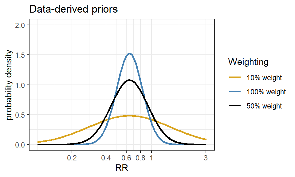
References
Goligher, Ewan C, George Tomlinson, David Hajage, Duminda N Wijeysundera, Eddy Fan, Peter Jüni, Daniel Brodie, Arthur S Slutsky, and Alain Combes. 2018. “Extracorporeal Membrane Oxygenation for Severe Acute Respiratory Distress Syndrome and Posterior Probability of Mortality Benefit in a Post Hoc Bayesian Analysis of a Randomized Clinical Trial.” Jama 320 (21): 2251–59.
Johnson, Sindhu R, George A Tomlinson, Gillian A Hawker, John T Granton, and Brian M Feldman. 2010. “Methods to Elicit Beliefs for Bayesian Priors: A Systematic Review.” Journal of Clinical Epidemiology 63 (4): 355–69.
Johnson, Sindhu R, George A Tomlinson, Gillian A Hawker, John T Granton, Haddas A Grosbein, and Brian M Feldman. 2010. “A Valid and Reliable Belief Elicitation Method for Bayesian Priors.” Journal of Clinical Epidemiology 63 (4): 370–83.
Lesaffre, Emmanuel, Gianluca Baio, and Bruno Boulanger. 2020. Bayesian Methods in Pharmaceutical Research. CRC Press.
Munshi, Laveena, Teagan Telesnicki, Allan Walkey, and Eddy Fan. 2014. “Extracorporeal Life Support for Acute Respiratory Failure. A Systematic Review and Metaanalysis.” Annals of the American Thoracic Society 11 (5): 802–10.
Noah, Moronke A, Giles J Peek, Simon J Finney, Mark J Griffiths, David A Harrison, Richard Grieve, M Zia Sadique, et al. 2011. “Referral to an Extracorporeal Membrane Oxygenation Center and Mortality Among Patients with Severe 2009 Influenza a (H1N1).” Jama 306 (15): 1659–68.
O’Hagan, Anthony, Caitlin E Buck, Alireza Daneshkhah, J Richard Eiser, Paul H Garthwaite, David J Jenkinson, Jeremy E Oakley, and Tim Rakow. 2006. “Uncertain Judgements: Eliciting Experts’ Probabilities.”
Peek, Giles J, Miranda Mugford, Ravindranath Tiruvoipati, Andrew Wilson, Elizabeth Allen, Mariamma M Thalanany, Clare L Hibbert, et al. 2009. “Efficacy and Economic Assessment of Conventional Ventilatory Support Versus Extracorporeal Membrane Oxygenation for Severe Adult Respiratory Failure (CESAR): A Multicentre Randomised Controlled Trial.” The Lancet 374 (9698): 1351–63.
Pham, Tài, Alain Combes, Hadrien Rozé, Sylvie Chevret, Alain Mercat, Antoine Roch, Bruno Mourvillier, et al. 2013. “Extracorporeal Membrane Oxygenation for Pandemic Influenza a (H1N1)–Induced Acute Respiratory Distress Syndrome: A Cohort Study and Propensity-Matched Analysis.” American Journal of Respiratory and Critical Care Medicine 187 (3): 276–85.
Spiegelhalter, David J. 2004. “Incorporating Bayesian Ideas into Health-Care Evaluation.” Statistical Science 19 (1): 156–74.
Spiegelhalter, David J., Keith R. Abrams, and Jonathan P. Myles. 2003. Bayesian Approaches to Clinical Trials and Health-Care Evaluation. John Wiley & Sons, Ltd. https://doi.org/10.1002/0470092602.