require(tidyverse)
library(brms)
library(bayesplot)
library(DT)
library(gtsummary)
library(knitr)
library(ggpubr)Tutorial 6
Hands-on exercise fitting Bayesian meta-regression for a binary outcome
What is meta-regression?
Meta-analysis pools effect estimates from multiple independent studies. Meta-regression extends this by modelling between-study heterogeneity as a function of study-level covariates. For binary outcomes, the standard approach is:
- Each study \(i\) reports events \(r_i\) out of trials \(n_i\)
- A hierarchical logistic model links study-level log-odds to a population mean and random study effects
- Study-level covariates (moderators) explain part of the heterogeneity in the overall effect
The Bayesian hierarchical meta-regression model
Let \(\theta_i = \text{logit}(p_i)\) be the study-specific log-odds:
\[r_i \mid p_i, n_i \sim \text{Binomial}(p_i, n_i)\]
\[\theta_i = \mu + \beta_1 x_{i1} + \ldots + \beta_k x_{ik} + u_i\]
\[u_i \sim N(0, \tau^2)\]
\[\mu \sim N(0, 5^2), \quad \beta_j \sim N(0, 1^2), \quad \tau \sim \text{half-}t(3, 0, 1)\]
- \(\mu\) is the overall log-odds when all moderators equal zero
- \(\beta_j\) is the meta-regression coefficient for moderator \(j\) (change in log-odds per unit change in \(x_j\))
- \(\tau\) is the residual between-study heterogeneity after accounting for moderators
- \(I^2\) and \(H^2\) summarize the fraction of total variability attributable to between-study heterogeneity
Example: BCG vaccine efficacy (metafor package)
The dat.bcg dataset from the metafor package [@viechtbauer2010conducting] contains 13 randomized trials of the BCG vaccine against tuberculosis. Each study reports TB cases in vaccinated and unvaccinated groups. A study-level covariate, absolute latitude, is hypothesized to moderate vaccine efficacy (higher latitudes = cooler climates where BCG is more effective).
library(metafor)

data(dat.bcg)

# Compute per-arm event counts
bcg <- dat.bcg %>%
  as_tibble() %>%
  transmute(
    study     = trial,
    author    = author,
    year      = year,
    latitude  = ablat,
    # Vaccinated arm
    r_vac     = tpos,
    n_vac     = tpos + tneg,
    # Control arm
    r_ctrl    = cpos,
    n_ctrl    = cpos + cneg,
    # Log risk ratio (for descriptive purposes)
    log_rr    = log((tpos / (tpos + tneg)) / (cpos / (cpos + cneg))),
    latitude_s = scale(ablat)[, 1]   # standardise for prior interpretability
  )

bcg %>%
  select(author, year, latitude, r_vac, n_vac, r_ctrl, n_ctrl, log_rr) %>%
  mutate(across(where(is.numeric), round, 3)) %>%
  datatable(rownames = FALSE,
            options = list(dom = 't', pageLength = 15,
                           columnDefs = list(
                             list(className = 'dt-center', targets = 0:7))))
Data structure for brms
We reshape into a long format: one row per arm per study, with a treatment indicator and outcome counts.
bcg_long <- bind_rows(
  bcg %>% transmute(study, author, year, latitude, latitude_s,
                    arm = "vaccinated", r = r_vac, n = n_vac),
  bcg %>% transmute(study, author, year, latitude, latitude_s,
                    arm = "control",    r = r_ctrl, n = n_ctrl)
) %>%
  mutate(
    vaccinated = as.integer(arm == "vaccinated"),
    study_f    = factor(study)
  ) %>%
  arrange(study, arm)

head(bcg_long, 6)
# A tibble: 6 × 10
study author year latitude latitude_s arm r n vaccinated study_f
<int> <chr> <int> <int> <dbl> <chr> <int> <int> <int> <fct>
1 1 Aronson 1948 44 0.730 cont… 11 139 0 1
2 1 Aronson 1948 44 0.730 vacc… 4 123 1 1
3 2 Ferguson… 1949 55 1.49 cont… 29 303 0 2
4 2 Ferguson… 1949 55 1.49 vacc… 6 306 1 2
5 3 Rosentha… 1960 42 0.591 cont… 11 220 0 3
6 3 Rosentha… 1960 42 0.591 vacc… 3 231 1 3 Prior specification and visualization
For the meta-regression we need priors on:
- \(\mu\): intercept (log-odds of TB in the control arm at mean latitude)
- \(\beta_\text{vac}\): main effect of vaccination (log-OR; our key estimand)
- \(\beta_\text{lat}\): moderation by latitude on the vaccination effect (interaction)
- \(\tau\): residual between-study SD on the log-odds scale
x_grid <- seq(-5, 5, by = 0.01)

p1 <- ggplot(tibble(x = x_grid, y = dnorm(x_grid, 0, 5)), aes(x, y)) +
  geom_line(colour = "steelblue", linewidth = 1) +
  labs(title = "Intercept prior: N(0, 5)",
       subtitle = "log-odds of TB in controls", x = "log-odds", y = "Density") +
  theme_bw()

p2 <- ggplot(tibble(x = x_grid, y = dnorm(x_grid, 0, 1)), aes(x, y)) +
  geom_line(colour = "tomato", linewidth = 1) +
  geom_vline(xintercept = c(-1.96, 1.96), linetype = "dashed", colour = "grey50") +
  annotate("text", x = -4.5, y = 0.35,
           label = paste0("OR 95% range:\n[",
                          round(exp(-1.96), 2), ", ", round(exp(1.96), 2), "]"),
           size = 2.8, hjust = 0) +
  labs(title = "Regression coeff prior: N(0, 1)",
       subtitle = "Vaccination + moderation log-ORs", x = "log-OR", y = "Density") +
  theme_bw()

p3 <- tibble(x = seq(0, 4, by = 0.01)) %>%
  ggplot(aes(x = x,
             y = 2 * dt(x / 1, df = 3) / 1)) +
  geom_line(colour = "darkgreen", linewidth = 1) +
  labs(title = "Between-study SD prior: half-t(3, 0, 1)",
       subtitle = "Residual heterogeneity tau", x = expression(tau), y = "Density") +
  theme_bw()

ggarrange(p1, p2, p3, nrow = 2)
$`1`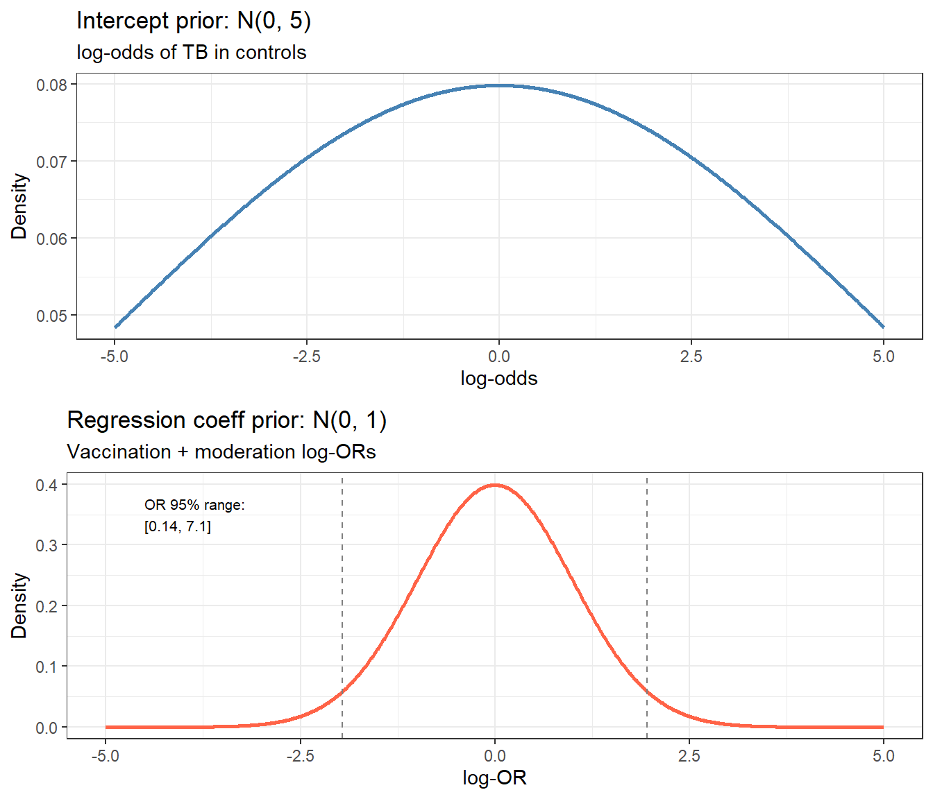
$`2`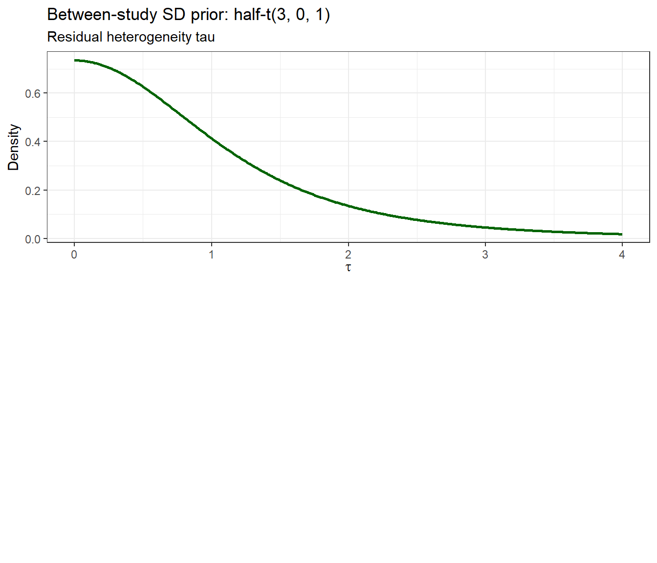
attr(,"class")
[1] "list"      "ggarrange"
Rationale for prior choices
- Intercept N(0, 5): log-odds scale - places 95% of mass between OR \(\approx\) 0.004 and 268, essentially non-informative about the baseline TB risk.
- Regression coefficients N(0, 1): on the log-OR scale, a 95% interval of \([-1.96, 1.96]\) corresponds to ORs between 0.14 and 7.4 - scientifically plausible for a vaccine effect or a moderator.
- \(\tau \sim\) half-t(3, 0, 1): a weakly informative prior on between-study SD, following recommendations for meta-analysis [@rover2021weakly]. It allows considerable heterogeneity while regularizing extreme values.
Fit the Bayesian meta-regression model
The model includes:
- A random study-level intercept (to capture baseline log-odds heterogeneity)
- A fixed effect of vaccination
- An interaction between vaccination and latitude (the moderator)
fit_meta <- brm(
  r | trials(n) ~ vaccinated + vaccinated:latitude_s + (1 | study_f),
  data    = bcg_long,
  family  = binomial(link = "logit"),
  prior   = c(
    prior(normal(0, 5), class = "Intercept"),
    prior(normal(0, 1), class = "b"),
    prior(student_t(3, 0, 1), class = "sd")
  ),
  iter    = 8000,
  warmup  = 4000,
  chains  = 4,
  cores   = 4,
  seed    = 123,
  silent  = 2,
  refresh = 0
)

saveRDS(fit_meta, "data/chp9_meta_bcg")
fit_meta <- readRDS("data/chp9_meta_bcg")
summary(fit_meta) Family: binomial
Links: mu = logit
Formula: r | trials(n) ~ vaccinated + vaccinated:latitude_s + (1 | study_f)
Data: bcg_long (Number of observations: 26)
Draws: 4 chains, each with iter = 8000; warmup = 4000; thin = 1;
total post-warmup draws = 16000
Group-Level Effects:
~study_f (Number of levels: 13)
Estimate Est.Error l-95% CI u-95% CI Rhat Bulk_ESS Tail_ESS
sd(Intercept) 1.62 0.33 1.11 2.41 1.00 2699 5285
Population-Level Effects:
Estimate Est.Error l-95% CI u-95% CI Rhat Bulk_ESS
Intercept -4.11 0.46 -5.03 -3.19 1.00 2502
vaccinated -0.71 0.05 -0.81 -0.62 1.00 9019
vaccinated:latitude_s -0.48 0.04 -0.56 -0.40 1.00 9145
Tail_ESS
Intercept 3262
vaccinated 9436
vaccinated:latitude_s 9499
Draws were sampled using sampling(NUTS). For each parameter, Bulk_ESS
and Tail_ESS are effective sample size measures, and Rhat is the potential
scale reduction factor on split chains (at convergence, Rhat = 1).Model diagnostics
plot(fit_meta, variable = c("b_Intercept", "b_vaccinated",
                             "b_vaccinated:latitude_s", "sd_study_f__Intercept"))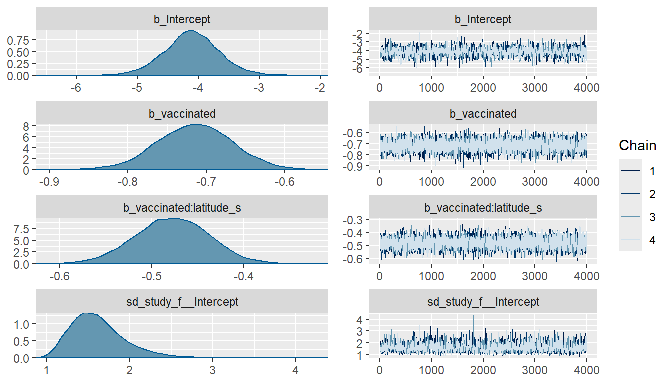
pp_check(fit_meta, ndraws = 100) +
  labs(title = "Posterior predictive check - meta-regression") +
  theme_bw()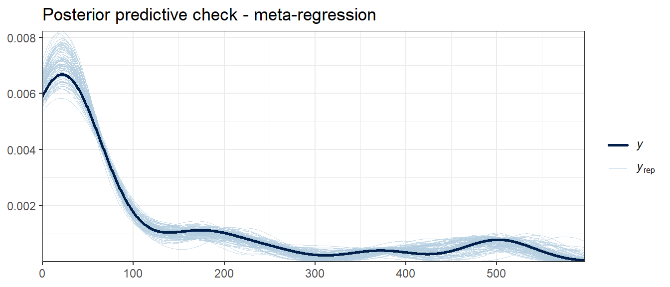
Posterior vaccine effect and moderation by latitude
Overall vaccine log-OR
draws_meta <- as_draws_df(fit_meta)

# Posterior of the vaccine log-OR (at mean latitude, latitude_s = 0)
vac_logOR <- draws_meta$b_vaccinated

ggplot(tibble(logOR = vac_logOR), aes(x = logOR)) +
  geom_density(fill = "steelblue", alpha = 0.5) +
  geom_vline(xintercept = 0, linetype = "dashed") +
  geom_vline(xintercept = quantile(vac_logOR, c(0.025, 0.975)),
             linetype = "dotted", colour = "tomato") +
  labs(title = "Posterior distribution of vaccine log-OR (at mean latitude)",
       x = "log-OR (vaccinated vs control)", y = "Density") +
  theme_bw()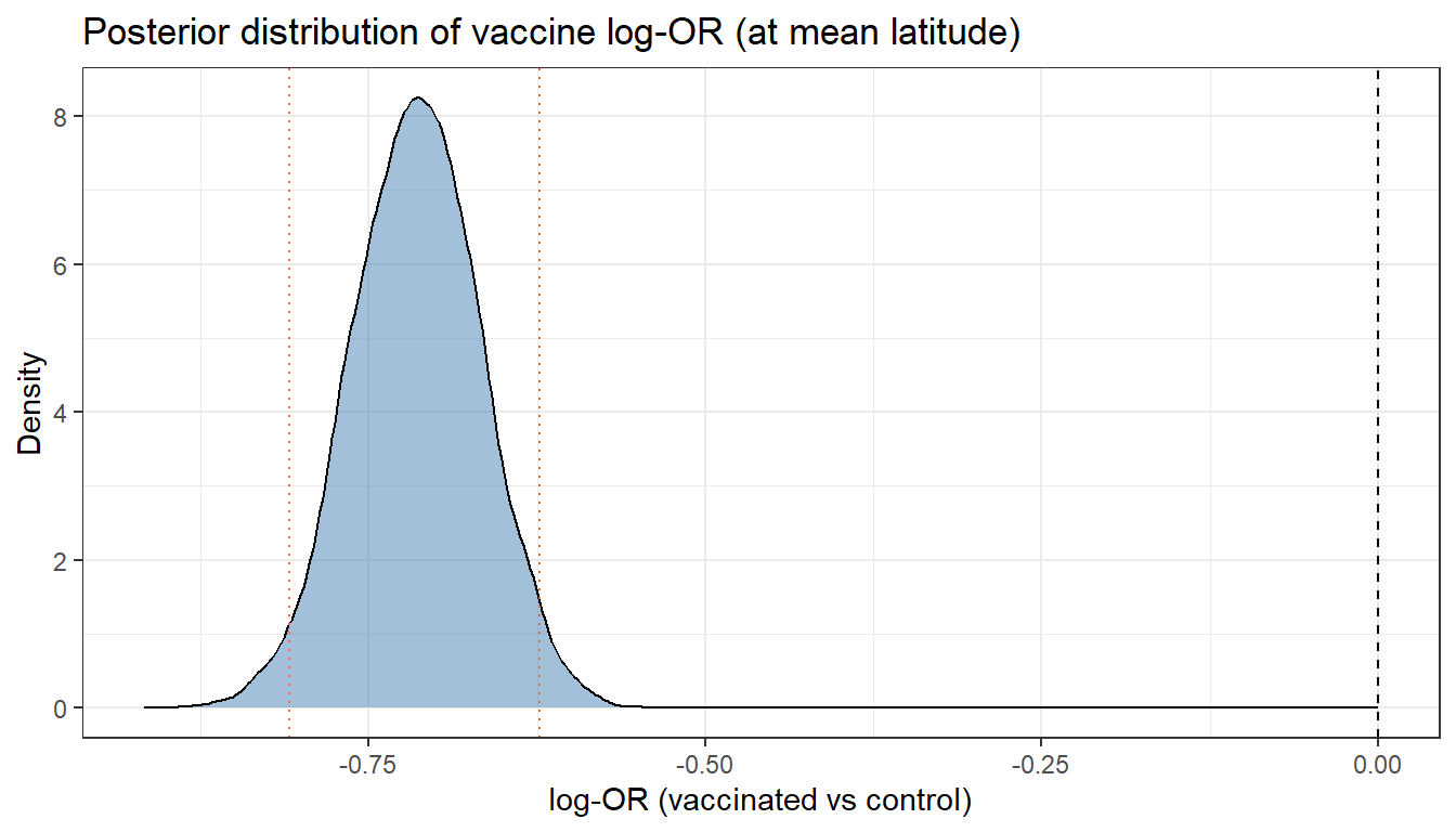
cat("Vaccine log-OR (mean latitude):\n")Vaccine log-OR (mean latitude):cat(" Mean:", round(mean(vac_logOR), 3), "\n") Mean: -0.715 cat(" 95% CrI: [", round(quantile(vac_logOR, 0.025), 3), ",",
round(quantile(vac_logOR, 0.975), 3), "]\n") 95% CrI: [ -0.809 , -0.623 ]cat(" Posterior OR:", round(exp(mean(vac_logOR)), 3), "\n") Posterior OR: 0.489 cat(" P(OR < 1):", round(mean(vac_logOR < 0), 3), "\n") P(OR < 1): 1 Moderation by latitude
lat_mod <- draws_meta$`b_vaccinated:latitude_s`

ggplot(tibble(mod = lat_mod), aes(x = mod)) +
  geom_density(fill = "goldenrod", alpha = 0.5) +
  geom_vline(xintercept = 0, linetype = "dashed") +
  geom_vline(xintercept = quantile(lat_mod, c(0.025, 0.975)),
             linetype = "dotted", colour = "tomato") +
  labs(title = "Posterior: interaction of vaccine effect and latitude",
       subtitle = "Negative = stronger protection at higher latitudes",
       x = "log-OR per SD of latitude", y = "Density") +
  theme_bw()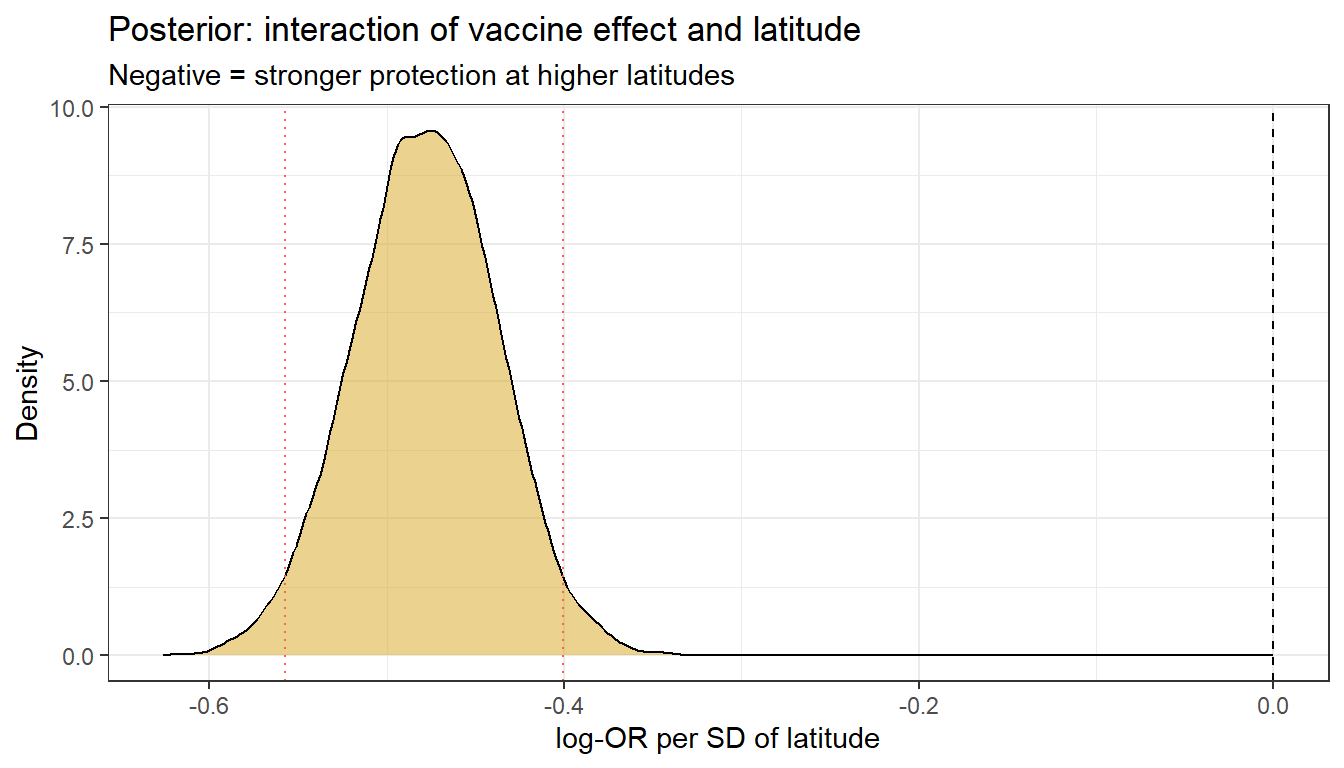
cat("Latitude moderation coefficient:\n")Latitude moderation coefficient:cat(" Mean:", round(mean(lat_mod), 3), "\n") Mean: -0.478 cat(" 95% CrI: [", round(quantile(lat_mod, 0.025), 3), ",",
round(quantile(lat_mod, 0.975), 3), "]\n") 95% CrI: [ -0.558 , -0.401 ]cat(" P(moderation < 0):", round(mean(lat_mod < 0), 3), "\n") P(moderation < 0): 1 Vaccine effect across the latitude gradient
lat_seq <- seq(min(bcg$latitude_s), max(bcg$latitude_s), length.out = 50)
lat_raw <- lat_seq * sd(bcg$latitude) + mean(bcg$latitude)

# For each posterior draw: vaccine log-OR at each latitude
or_lat <- sapply(lat_seq, function(ls) {
  draws_meta$b_vaccinated + draws_meta$`b_vaccinated:latitude_s` * ls
})
# dim: (n_draws x 50)

or_summary <- apply(or_lat, 2, quantile, probs = c(0.025, 0.5, 0.975)) %>%
  t() %>%
  as.data.frame() %>%
  setNames(c("lower", "median", "upper")) %>%
  mutate(latitude = lat_raw)

ggplot(or_summary, aes(x = latitude, y = median)) +
  geom_ribbon(aes(ymin = lower, ymax = upper), fill = "steelblue", alpha = 0.3) +
  geom_line(colour = "steelblue", linewidth = 1) +
  geom_hline(yintercept = 0, linetype = "dashed", colour = "grey50") +
  geom_point(data = bcg, aes(x = latitude, y = log_rr),
             colour = "black", size = 2) +
  labs(title = "BCG vaccine log-OR as a function of latitude",
       subtitle = "Ribbon = 95% credible band; points = study-specific log-RR",
       x = "Absolute latitude (degrees)", y = "Vaccine log-OR") +
  theme_bw()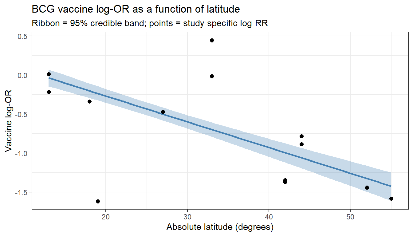
Between-study heterogeneity
- Nakagawa, S. & Schielzeth, H. (2013). A general and simple method for obtaining \(R^2\) from generalized linear mixed-effects models. Methods in Ecology and Evolution, 4(2), 133-142.
tau_draws <- draws_meta$sd_study_f__Intercept

ggplot(tibble(tau = tau_draws), aes(x = tau)) +
  geom_density(fill = "tomato", alpha = 0.5) +
  geom_vline(xintercept = quantile(tau_draws, c(0.025, 0.975)),
             linetype = "dashed", colour = "grey30") +
  labs(title = expression("Posterior distribution of between-study SD " * tau),
       x = expression(tau ~ "(log-odds scale)"), y = "Density") +
  theme_bw()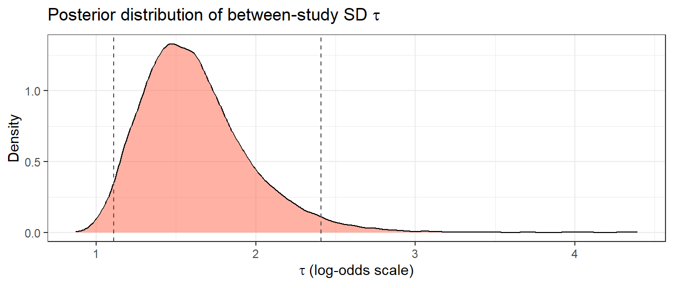
cat("Between-study tau:\n")Between-study tau:cat(" Mean:", round(mean(tau_draws), 3), "\n") Mean: 1.619 cat(" 95% CrI: [", round(quantile(tau_draws, 0.025), 3), ",",
round(quantile(tau_draws, 0.975), 3), "]\n") 95% CrI: [ 1.111 , 2.408 ]# Exact I^2 for binomial-logistic hierarchical model
# pi^2/3 is the variance of the logistic distribution -
# the theoretical within-study variance on the log-odds scale
I2_draws <- tau_draws^2 / (tau_draws^2 + (pi^2 / 3))
H2_draws <- (tau_draws^2 + (pi^2 / 3)) / (pi^2 / 3)
cat(" I^2 (mean):", round(mean(I2_draws), 3), "\n") I^2 (mean): 0.436 cat(" I^2 95% CrI: [", round(quantile(I2_draws, 0.025), 3), ",",
round(quantile(I2_draws, 0.975), 3), "]\n") I^2 95% CrI: [ 0.273 , 0.638 ]cat(" H^2 (mean):", round(mean(H2_draws), 3), "\n") H^2 (mean): 1.831 cat(" H^2 95% CrI: [", round(quantile(H2_draws, 0.025), 3), ",",
round(quantile(H2_draws, 0.975), 3), "]\n") H^2 95% CrI: [ 1.375 , 2.763 ]Forest plot of study-specific effects
# For each study, predict log-odds for vaccinated = 1 and vaccinated = 0, including the study-specific random effect.

studies <- bcg %>% select(study, author, latitude, latitude_s) %>%
  mutate(study_f = factor(study))

study_logOR_draws <- lapply(seq_len(nrow(studies)), function(i) {

  nd_vac  <- data.frame(
    vaccinated  = 1,
    latitude_s  = studies$latitude_s[i],
    study_f     = studies$study_f[i],
    n           = 1   # required by trials(n) in the formula
  )
  nd_ctrl <- data.frame(
    vaccinated  = 0,
    latitude_s  = studies$latitude_s[i],
    study_f     = studies$study_f[i],
    n           = 1
  )

  lp_vac  <- posterior_linpred(fit_meta, newdata = nd_vac,
                                re_formula = NULL, transform = FALSE)
  lp_ctrl <- posterior_linpred(fit_meta, newdata = nd_ctrl,
                                re_formula = NULL, transform = FALSE)

  as.numeric(lp_vac - lp_ctrl)
})

# Summarise: posterior mean and 95% CrI per study
study_effects <- tibble(
  author   = studies$author,
  latitude = studies$latitude,
  logOR    = sapply(study_logOR_draws, mean),
  lower    = sapply(study_logOR_draws, quantile, probs = 0.025),
  upper    = sapply(study_logOR_draws, quantile, probs = 0.975)
) %>%
  arrange(logOR)

# Pooled posterior vaccine log-OR (at mean latitude, latitude_s = 0)
pool_logOR <- mean(draws_meta$b_vaccinated)
pool_lower <- quantile(draws_meta$b_vaccinated, 0.025)
pool_upper <- quantile(draws_meta$b_vaccinated, 0.975)

ggplot(study_effects,
       aes(x = exp(logOR), y = reorder(author, logOR))) +
  geom_point(size = 3, colour = "steelblue") +
  geom_errorbarh(aes(xmin = exp(lower), xmax = exp(upper)),
                 height = 0.3, colour = "steelblue") +
  geom_vline(xintercept = exp(pool_logOR),
             linetype = "solid", colour = "tomato", linewidth = 0.9) +
  annotate("rect",
           xmin = exp(pool_lower), xmax = exp(pool_upper),
           ymin = -Inf, ymax = Inf,
           alpha = 0.12, fill = "tomato") +
  geom_vline(xintercept = 1, linetype = "dashed", colour = "grey40") +
  scale_x_log10(breaks = c(0.05, 0.1, 0.2, 0.5, 1, 2)) +
  labs(title = "Bayesian forest plot: BCG vaccine vs control",
       subtitle = paste0(
         "Red line = pooled posterior OR (at mean latitude) = ",
         round(exp(pool_logOR), 2),
         " [", round(exp(pool_lower), 2), ", ",
         round(exp(pool_upper), 2), "]\n"
       ),
       x = "Odds Ratio (log scale)", y = NULL) +
  theme_bw()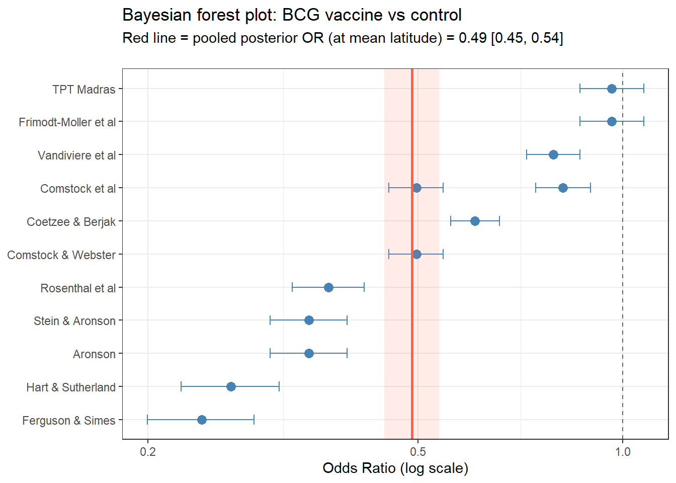
Summary: Bayesian meta-regression for binary outcomes
- The hierarchical binomial-logistic model naturally handles between-study heterogeneity via a random intercept (\(\tau\)).
- Meta-regression coefficients (\(\beta_\text{lat}\)) quantify how much of the heterogeneity is explained by study-level moderators.
- Weakly informative priors on \(\tau\) and regression coefficients prevent implausible estimates in small meta-analyses.
- The Bayesian posterior provides direct probability statements: e.g., \(P(\text{OR} < 1) = 0.99\), or \(P(\tau > 0.5) = 0.15\).
- Residual \(\tau\) after accounting for moderators tells us whether identified moderators fully explain heterogeneity.