Week 1 - Plotting probability density function in R

1. Hands-on excerise plotting four common distributions in R

require(tidyverse)

1.1 Uniform distribution

First setting up parameters: for UNIF(0,1), a=0 and b=1.
Let x represents the random variable that follows UNIF(0,1), we create a vector that hosts a sequence of values for x that range between a=0 (min) and b=1 (max) to form the x-axis of the pdf plot.
We then obtain probability density vector labelled y for each value in the x sequence from a UNIF(0,1) distribution in R.
Creating a dataframe that combines x and y and use ggplot to create the pdf plot.

# setting up distribution parameters;
a=0; b=1
# creating x vector;
x <- seq(from = 0, to = 1, by = 0.001)
# finding density probability for each x element;
y <- dunif(x, min = a, max = b)
# create a plotting dataframe;
data <- data.frame(x,y)
# ggplot;
ggplot(data, aes(x=x, y=y)) +
  geom_line() +
  labs(x='X', y='density', title='PDF of Uniform(0,1)') +
  theme_bw()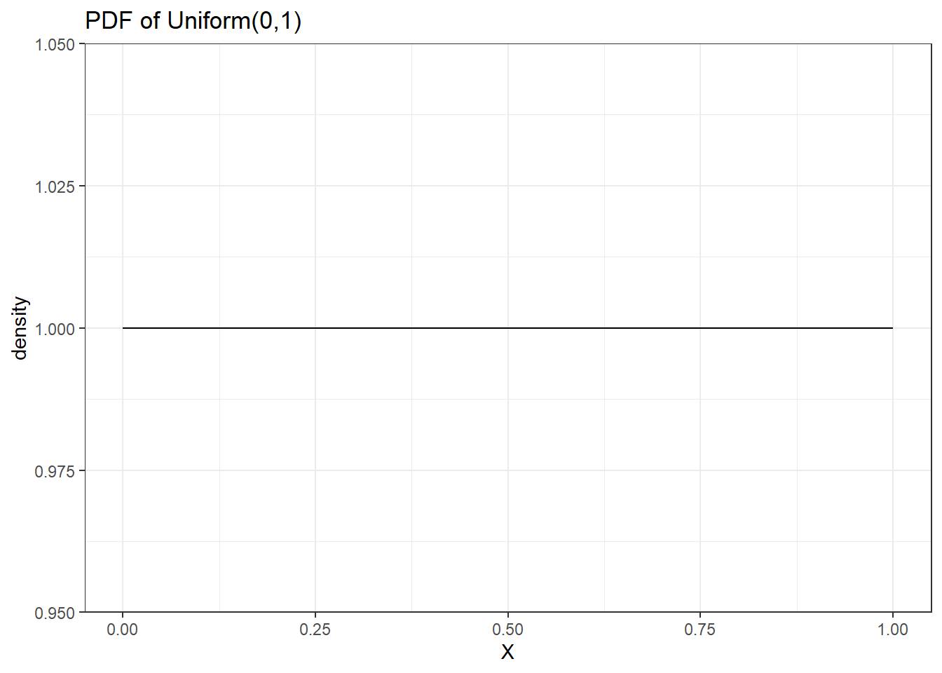

How can we improve the plot to show the box shape?

# setting up distribution parameters;
a=0; b=1
# creating x vector;
x <- seq(from = -0.1, to = 1.1, by = 0.001) #given more range to x-axis eventhough we know the density for x<0 and x>1 is zero!;
# finding density probability for each x element;
y <- dunif(x, min = a, max = b)
# create a plotting dataframe;
data <- data.frame(x,y)
# ggplot;
ggplot(data, aes(x=x, y=y)) +
  geom_line() +
  labs(x='X', y='density', title='PDF of Uniform(0,1)') +
  theme_bw()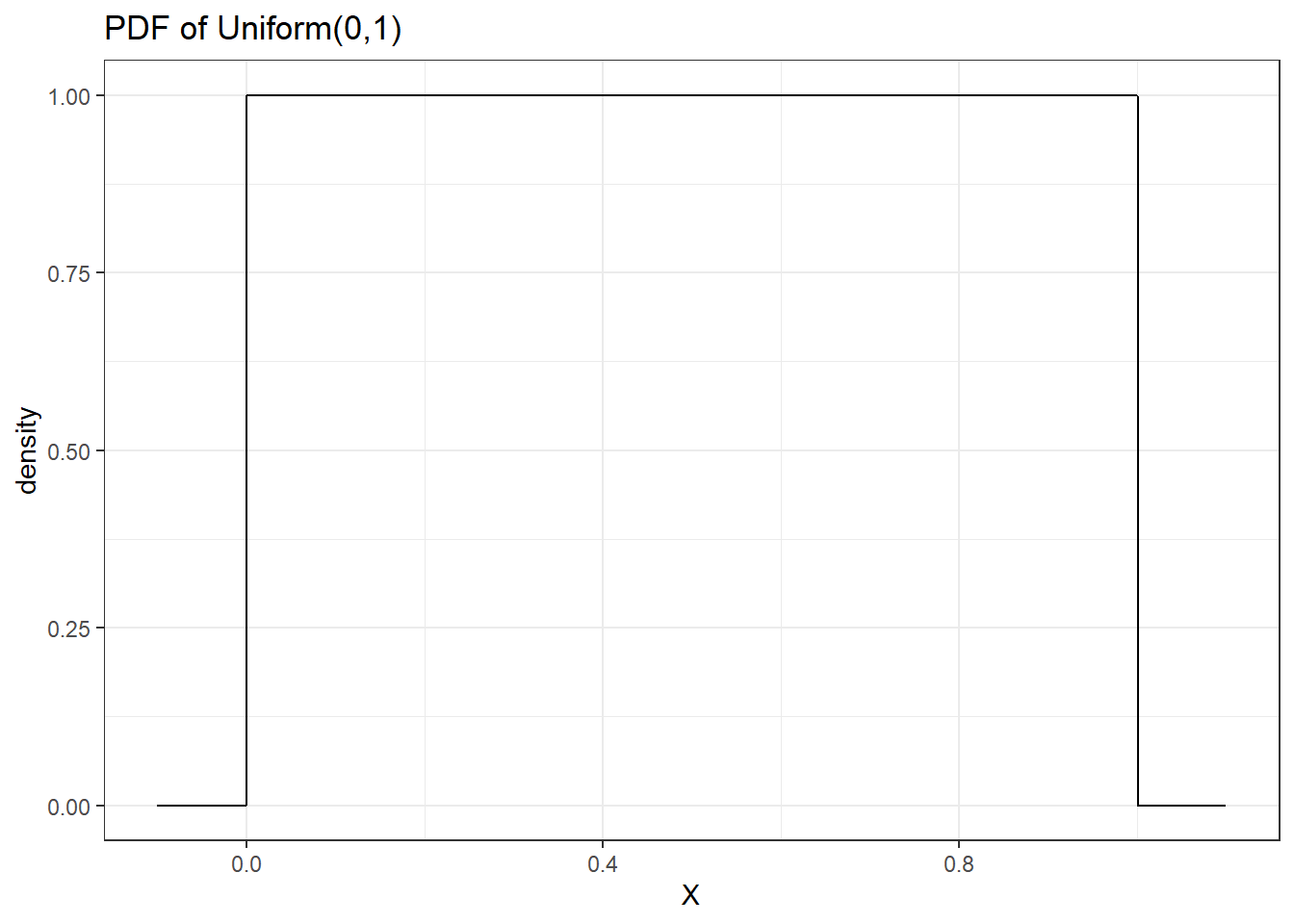

Figure 2: Uniform distribution (0,1) with extended x range

Now try it yourself

Plotting UNIF(1,2) in R

1.2 Normal distribution

First setting up parameters: for Normal(0,1), mean=0 and sd=1.
Let x represents the random variable that follows Normal(0,1), we create a vector that hosts a sequence of values for x that range between \(min=(0-4\times sd)\) and \(min=(0+4\times sd)\) to form the x-axis of the pdf plot.
We then obtain probability density vector labelled y for each value in the x sequence from N(0,1).
Creating a dataframe that combines x and y and use ggplot to create the pdf plot.

# setting up distribution parameters;
mean=0; sd=1
# creating x vector;
x <- seq(from = (mean-4*sd), to = (mean+4*sd), by = 0.001)
# finding density probability for each x element;
y <- dnorm(x, mean=mean, sd=sd)
# create a plotting dataframe;
data <- data.frame(x,y)
# ggplot;
ggplot(data, aes(x=x, y=y)) +
  geom_line() +
  labs(x='X', y='density', title='PDF of N(0,1)') +
  theme_bw()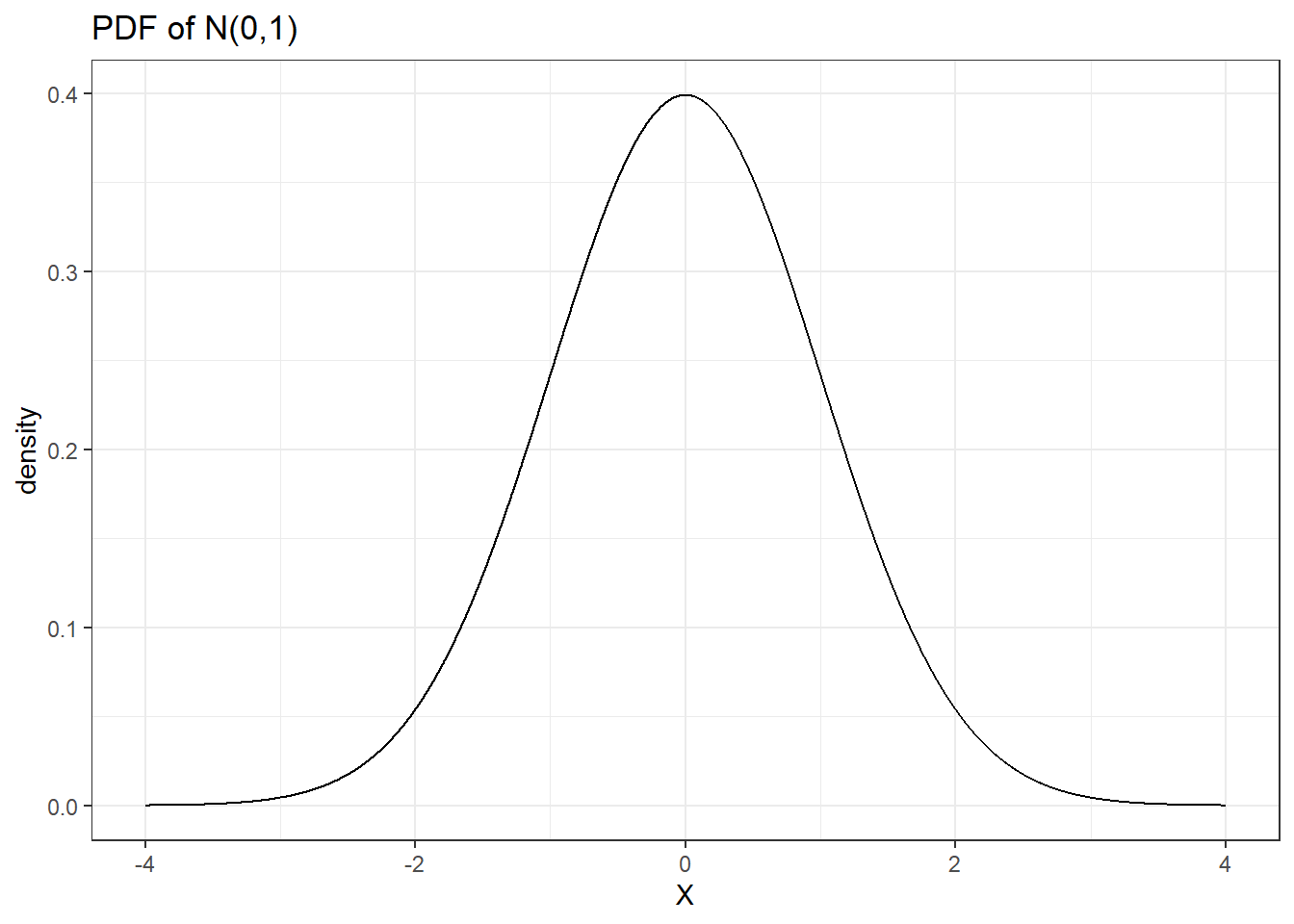

What is the probability under the curve for x < 0 while \(x \sim N(0,1)\), what about for x > 1.96?

pnorm(q=0, mean=0, sd=1, lower.tail = TRUE)

[1] 0.5

pnorm(q=1.96, mean=0, sd=1, lower.tail = FALSE)

[1] 0.0249979

Adding shaded area on the density plot.

# setting up distribution parameters;
mean=0; sd=1
# creating x vector;
x <- seq(from = (mean-4*sd), to = (mean+4*sd), by = 0.001)
# finding density probability for each x element;
y <- dnorm(x, mean=mean, sd=sd)
# create a plotting dataframe;
data <- data.frame(x,y)
# ggplot;
ggplot(data, aes(x=x, y=y)) +
  geom_line() +
  geom_area(data=data %>% filter(x < 0), fill='grey', alpha=.4) +
    geom_area(data=data %>% filter(x > 1.96), fill='red', alpha=.4) +
  labs(x='X', y='density', title='PDF of N(0,1)') +
  theme_bw()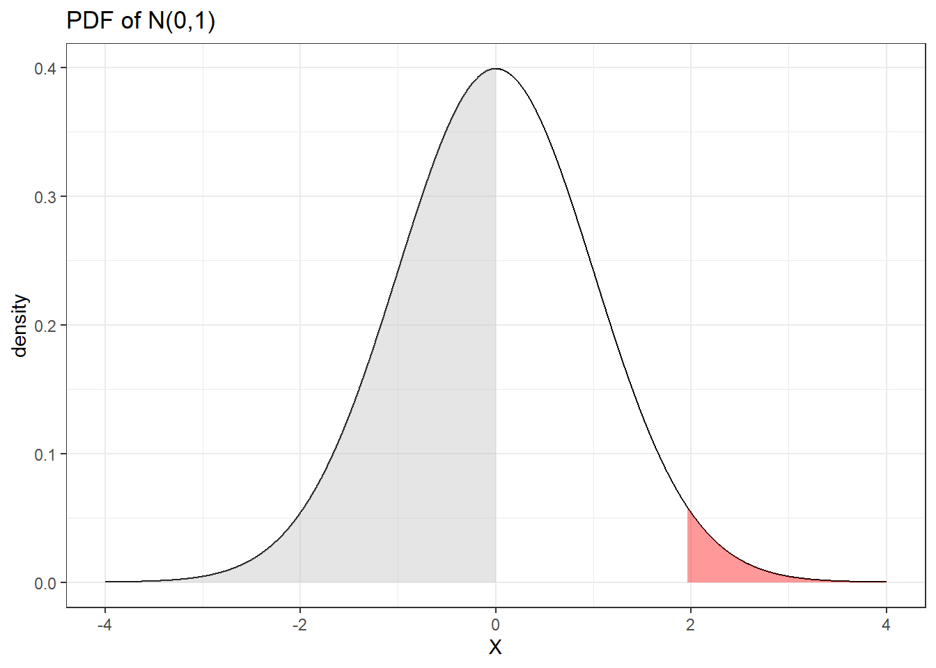

Now try it yourself

Plotting N(1,2) in R. If \(x \sim N(1,2)\), please find \(P(x>2)\).

1.3 Beta distribution and Gamma distribution

Giving the example codes above, can you plot Beta(2,2) and Gamma(5,1)?
The first step is to set up your parameters in R, then you have to create a sequence of x variables representing a plausible range of the random variable that will be latter used as the x-axis in the plot. Upon creating the x vector, you then obtain density probabilites from the target distribution using the r ddist() function.

# setting up distribution parameters;
shape1=1; shape2=1
# creating x vector;
x <- seq(from = 0, to = 1, by = 0.001)
# finding density probability for each x element;
y <- dbeta(x, shape1 = shape1, shape2 = shape2)
# create a plotting dataframe;
data <- data.frame(x,y)
# ggplot;
ggplot(data, aes(x=x, y=y)) +
  geom_line() +
  labs(x='X', y='density', title='PDF of Beta(1,1)') +
  theme_bw()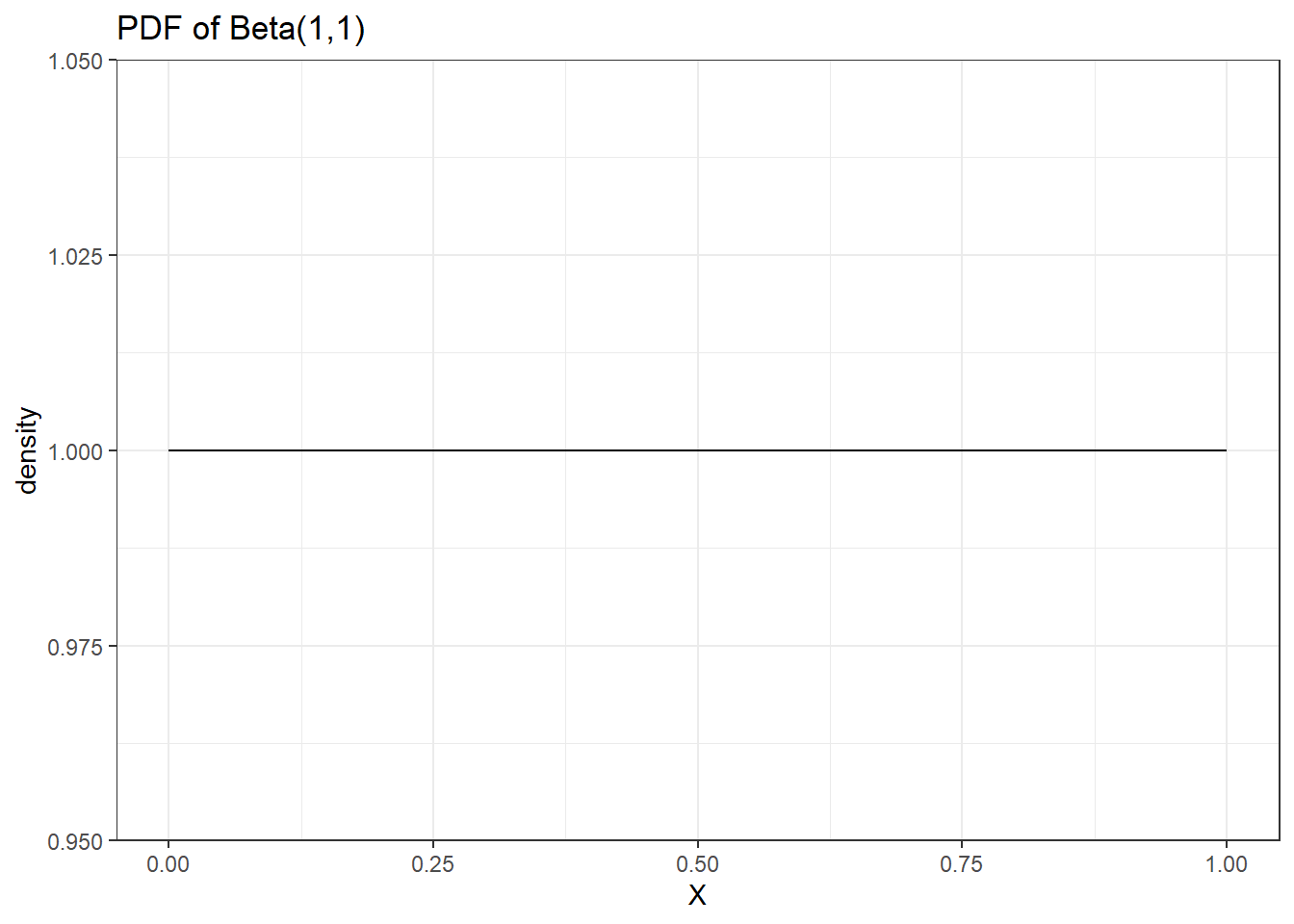

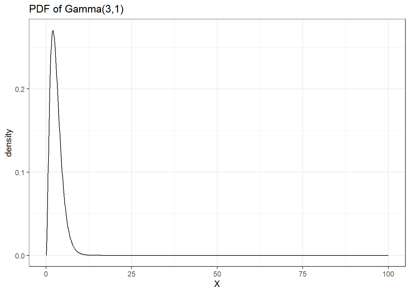
# setting up distribution parameters;
shape=3; rate=1
# creating x vector;
x <- seq(from = 0, to = 100, by = 0.1)
# finding density probability for each x element;
y <- dgamma(x, shape=shape, rate=rate)
# create a plotting dataframe;
data <- data.frame(x,y)
# ggplot;
ggplot(data, aes(x=x, y=y)) +
  geom_line() +
  labs(x='X', y='density', title='PDF of Gamma(3,1)') +
  theme_bw()