Bayesian Poisson regression

Learning Objectives

Learn how to fit Bayesian poisson and negative binomial regression with brms
Understand how to interpret and report regression posterior results

Models for Count Data

Example Count Data
- Number of deaths in cohort followed up for 5 years
- Number of deaths in subgroups of this cohort
- Number of episodes of cold or flu experienced by an individual in a year
- Number of hospitalizations a person experiences in a year

Poisson Distribution

If we count the number of events that occur over a fixed time period, this random variable Y can take on one of the whole numbers 0, 1, 2,…
Let \(\theta = E(Y)\), then the probability of observing \(y\) events (probability mass function) is

\[ P(Y = y \mid \theta) = \frac{\theta^y \exp(-\theta)}{y!}, y = 0,1,2, \ldots\]

There is only one parameter, the mean (or expected number of events)
This same parameter is also the variance

\[\theta = E(Y) = Var(Y)\]

If we know the length of follow-up time is T, then we can write the expected number \(\theta\) as

\[\theta = \lambda \times T\]

where \(\lambda\) is the rate per unit of time.

Then we can replace the mean by rate \(\times\) time in the Poisson probability mass function:

\[P(Y = y \mid \lambda, T) = \frac{(\lambda T)^y \exp(-\lambda T)}{y!}, y = 0,1,2, \ldots\]

When to use Poisson Distribution
1. Time period of observation is known
2. The event can be counted in whole numbers
3. Occurrences are independent, so that one occurrence neither diminishes nor increases the chance of another
4. The rate of occurrence for the time period in question is constant
For rare events (small \(p\), large \(n\)), \(Y \sim Bin(p,n)\) has approximately Poisson distribution.
Not necessary to count how many events have not occurred: e.g. we cannot count how many episodes of flu did not occur

Modelling Rates

We are interested in factors that affect their rates, not their enrolment or follow-up times.

1. Simple Poisson Model (one-sample)

Suppose we have follow up time \(T_i\) and number of events \(Y_i\) for each subject
Lets assume that the underlying rate of events is the same for everyone
We are interested in this common underlying rate of events \(\lambda\)
We prefer to model \(\log(\lambda)\), where

\[ \lambda > 0 \leftrightarrow - \infty < \log(\lambda) < \infty\]

and

\[Y_i \sim Poisson(\theta_i)\] \[\theta_i = \lambda \times T_i\] \[\log(\lambda) = \alpha\]

\(\alpha\) is the log rate; \(\exp(\alpha)\) is the rate (on its original scale).

2. Two-sample Poisson Model (treatment vs control groups)

Now if we assume the underlying rate of events is not the same for everyone and that it’s associated with some covariates (e.g., treatment)
- Interested in the effect of treatment (\(TRT_i=0 , 1\))
Assume a rate \(\lambda_i\) that depends on the treatment received by subject \(i\), our model updated to

\[Y_i \sim Poisson(\theta_i)\] \[\theta_i = \lambda_i \times T_i\] \[\log(\lambda_i) = \alpha + \beta \times TRT_i\]

Given the model above, we can compare rate between treated (t) and controls (c)
- Observe \(Y_c\) events in 110 person-years in the control group

\[Y_c \sim Poisson(\theta_c)\] \[\theta_c = \lambda_c \times 110 \] \[\log(\lambda_c) = \alpha\] - Observe \(Y_t\) events in 100 person-years in the treated group

\[Y_t \sim Poisson(\theta_t)\] \[\theta_t = \lambda_t \times 100 \] \[\log(\lambda_t) = \alpha + \beta\]

Comparing the two models we have

\[\log(\lambda_t) - \log(\lambda_c) = \log(\frac{\lambda_t}{\lambda_c}) = \beta\]

where \(\beta\) is interpreted as log rate ratio.

The concept of “offset”

In this example, the Observe \(Y_c\) events in 110 person-years in the control group

\[\theta_c = \lambda_c \times 110 \] \[\log(\theta_c) = \log(\lambda_c) + \log(110) \]

and more generally we have

\[Y_i \sim Poisson(\theta_i)\]

\[\theta_i = \lambda \times T_i\] \[\log(\theta_i) = \log(\lambda_i) + \log(T_i)\] \[\log(\lambda_i) = \alpha + \beta \times TRT_i\]

The natural log of time (\(\log (T_i)\)) is is passed as the “offset” in brm (Bayesian model), glm and glmer models (frequentist model) for count data in R
We don’t estimate a parameter for the effect of log time - it is treated differently from other predictors (like age, for example)
It is the log(rate), not the log(mean) that is modelled linearly by the predictors
If the times are all equal to the same value TIME for participants, the offset can be omitted and the effects are for the rate per TIME

#example code for Poisson regression in brms;
brm(y ~ 1 + offset(log(Time)),
    data = dat,
    family = "poisson",
    prior = c(prior(normal(0, 100), class = "Intercept")),
    chains = 4,
    iter = 10000,
    warmup = 8000,
    cores = 4)

Poisson regression model

Consider the poisson regression model on \(Y\) with covariates \(X_1, \ldots, X_p\) and offset \(T\) (time), where

\[ Y_i \mid \beta_0, \beta_1, \ldots, \beta_p \sim Pois(\lambda_i T_i)\]

\[ \log(\lambda_i) = \beta_0 + \beta_1 X_{i1} + \ldots + \beta_p X_{ip}\]

The regression coefficients can be interpreted as log relative risk.
Furthermore, we can recalculate expected number of event over a period of time \(T\) using the exponential function,

\[\lambda_i \times T = \exp(\beta_0 + \beta_1 X_{i1} + \ldots + \beta_p X_{ip}) \times T\]

Assumptions of logistic regression models
1. Independent observations. This assumption can be modified if working with clustered data.
2. Linear relationship between continuous covariates and log-rate
3. No over-dispersion For Poisson distributed variable, we have its mean equals to its variance. Thus, conditioning on predictors \(X\), the expected value of \(Y\) should be roughly equivalent to the variability in \(Y\). If this assumption is violated, we can consider fitting a negative binomial regression model by allowing the variance to be different (larger) from the mean. We can use waic and loo to determine if the negative binomial model is of better fit than the Poisson model.
4. No zero-inflation When we observe majority of our study subjects with zero number of events over time, we call this data with an excess number of zeroes (zero-inflation). When we have excess zeroes in our count data, we can consider fitting a zero-inflated Poisson or a zero-inflated negative binomial regression model. We can use loo to determine if the zero-inflated models are of better fit than the Poisson model.
  - e.g., the number of hospitalizations a health 20-25 years old person experiences in a year
5. Multicollinearity Multicollinearity is the phenomenon when a number of the explanatory variables are strongly correlated.
6. Correctly specified regression model We can use posterior predictive distribution to check for regression fit between different models and can also use WAIC and LOO to compare them.

Modelling Falls and Fall-Related Injuries in Older Dialysis Patients in brms

This example is taken from (Cook et al. 2006). We included two covariates from the original data for demonstration purpose.
This is a dataset looking at the number of episodes of falling over a year by dialysis patients
Not all subjects had a full year of follow-up; some dropped out
We can account for different follow-up using a Poisson regression model with follow-up time as an “offset”.
To illustrate, we will use only two predictors: female sex, coded as 0/1, and history of previous falls, also coded as 0/1
- Displaying the first 10 observations:

Code

dat <- read.table("data/fallsData.txt",header=T, sep="")

dat %>%
  datatable(
  rownames = T,
  options = list(
    searching = FALSE,
    columnDefs = list(list(className = 'dt-center', 
                      targets = 0:3))))

First let’s examine the summary statistics

Code

dat %>% tbl_summary(
    statistic = list(all_continuous() ~ "{mean} ({sd})",
                     all_categorical() ~ "{n} / {N} ({p}%)"),
    digits = all_continuous() ~ 2)

Characteristic	N = 162¹
falls	1.54 (4.06)
fu	0.90 (0.21)
FemaleSex	70 / 162 (43%)
PrevFall	54 / 162 (33%)
¹ Mean (SD); n / N (%)

Code

# creating a subject ID;
dat$Subject <- factor(1:nrow(dat))

p1<-ggplot(dat, aes(x = falls)) + 
  geom_histogram(color = "white", breaks = seq(0, 40, by = 1)) +
  ggtitle("Histogram of the number of falls over a year")+
  ylab("frequency")+
  theme_bw()

p2<-ggplot(dat, aes(x = fu)) + 
  geom_histogram(color = "white", bins = 20) +
  ggtitle("Histogram of follow-up times")+
  ylab("frequency")+
  xlab("follow-up times")+
  theme_bw()

ggarrange(p1,p2, nrow=1, ncol = 2)

Now let choose priors using normal distribution. In this example, let’s consider informative priors!
1. It is unlikely that females have a fall rate less than 1/3 times or more than 3 times the rate in males

\[P(\frac{1}{3} < RR_{female} < 3) = 95\%\] \[P(\log(\frac{1}{3}) < log(RR_{female}) < log(3)) = 95\%\] \[\text{Prior Mean}(\log RR_{female}) = \frac{\log(\frac{1}{3})+log(3)}{2} = 0 \text{ (midpoint)}\] \[\text{Prior SD}(\log RR_{female}) = \frac{log(3) - \log(\frac{1}{3})}{1.96 \times 2} = 0.56 \] 2. Previous falls are a known risk factor for current falls, so we use a prior that puts most weight on \(RR_{prevfall}>1\)

\[P(0.75 < RR_{prevfall} < 4) = 95\%\] \[P(\log(0.75) < log(RR_{prevfall}) < log(4)) = 95\%\] \[\text{Prior Mean}(\log RR_{prevfall}) = \frac{\log(0.75)+log(3)}{2} = 0.55 \text{ (midpoint)}\] \[\text{Prior SD}(\log RR_{prevfall}) = \frac{log(4) - \log(0.75)}{1.96 \times 2} = 0.43 \]

Code

#sex;
s<-(log(3) - log(1/3))/(1.96*2)
m <- (log(3) + log(1/3))/2

p1<-data.frame(RR = seq(0,7,length=501)) %>%
  mutate(p = dlnorm(RR, meanlog = m, sdlog = s)) %>%
  mutate(Region = ifelse(RR<=1, "RR<1","RR>1"))%>%
  ggplot(aes(RR, p))+
  geom_line()+
  geom_area(aes(fill=Region),alpha=0.7)+
  theme_bw()+
  scale_fill_manual(values= c("goldenrod","steelblue"))+
  ggtitle(paste0("Prior RR for sex; P(RR<1)=",
                 round(100*plnorm(1,m,s)),"%"))+
  ylab("p(RR)")+
  scale_x_continuous(breaks=0:7)+
  theme_bw()

#previous falls
s<-(log(4) - log(0.75))/3.92
m <- (log(4) + log(0.75))/2

p2<-data.frame(RR = seq(0,7,length=501)) %>%
  mutate(p = dlnorm(RR, meanlog = m, sdlog = s)) %>%
  mutate(Region = ifelse(RR<=1, "RR<1","RR>1"))%>%
  ggplot(aes(RR, p))+
  geom_line()+
  geom_area(aes(fill=Region),alpha=0.7)+
  theme_bw()+
  scale_fill_manual(values= c("goldenrod","steelblue"))+
  ggtitle(paste0("Prior RR for prevfall; P(RR<1)=",
                 round(100*plnorm(1,m,s)),"%"))+
  ylab("p(RR)")+
  scale_x_continuous(breaks=0:7)+
  theme_bw()

ggarrange(p1,p2,nrow = 1, ncol=2)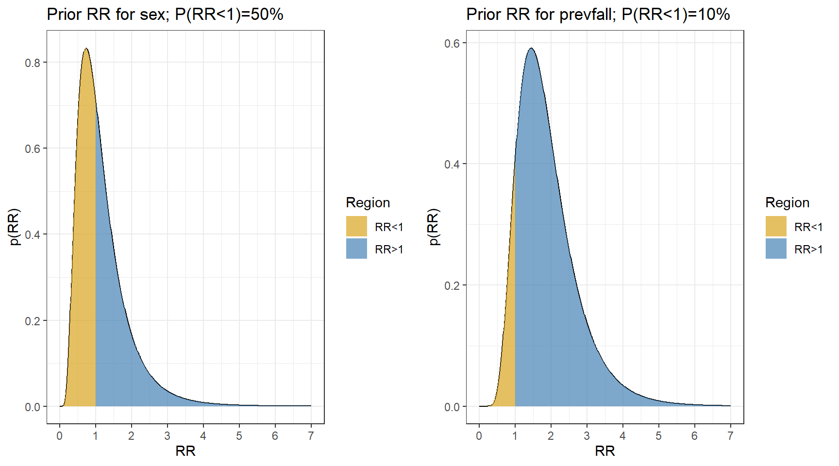

Model 1. Simple Poisson Model

model1 <- brm(falls ~ FemaleSex + PrevFall + offset(log(fu)),
    data = dat, 
    family = "poisson",
    sample_prior=T,
    prior = c(prior(normal(0, 100), class = "Intercept"),
              prior(normal(0, 0.56), class = "b", coef=FemaleSex),
              prior(normal(0.55, 0.43), class = "b", coef=PrevFall)),
    chains = 4, 
    iter = 7500, 
    warmup = 5000, 
    cores = 4,
    seed = 123, 
    silent = 2,
    refresh = 0)

# saveRDS(model1, "data/chap8_poisson_1")

Posterior summary

model1 <- readRDS("data/chap8_poisson_1")
plot(model1)

print(model1)

 Family: poisson 
  Links: mu = log 
Formula: falls ~ FemaleSex + PrevFall + offset(log(fu)) 
   Data: dat (Number of observations: 162) 
  Draws: 4 chains, each with iter = 7500; warmup = 5000; thin = 1;
         total post-warmup draws = 10000

Regression Coefficients:
          Estimate Est.Error l-95% CI u-95% CI Rhat Bulk_ESS Tail_ESS
Intercept     0.21      0.11    -0.01     0.41 1.00     6937     6087
FemaleSex    -0.54      0.13    -0.80    -0.27 1.00     7106     6678
PrevFall      1.10      0.12     0.86     1.35 1.00     7162     7060

Draws were sampled using sampling(NUTS). For each parameter, Bulk_ESS
and Tail_ESS are effective sample size measures, and Rhat is the potential
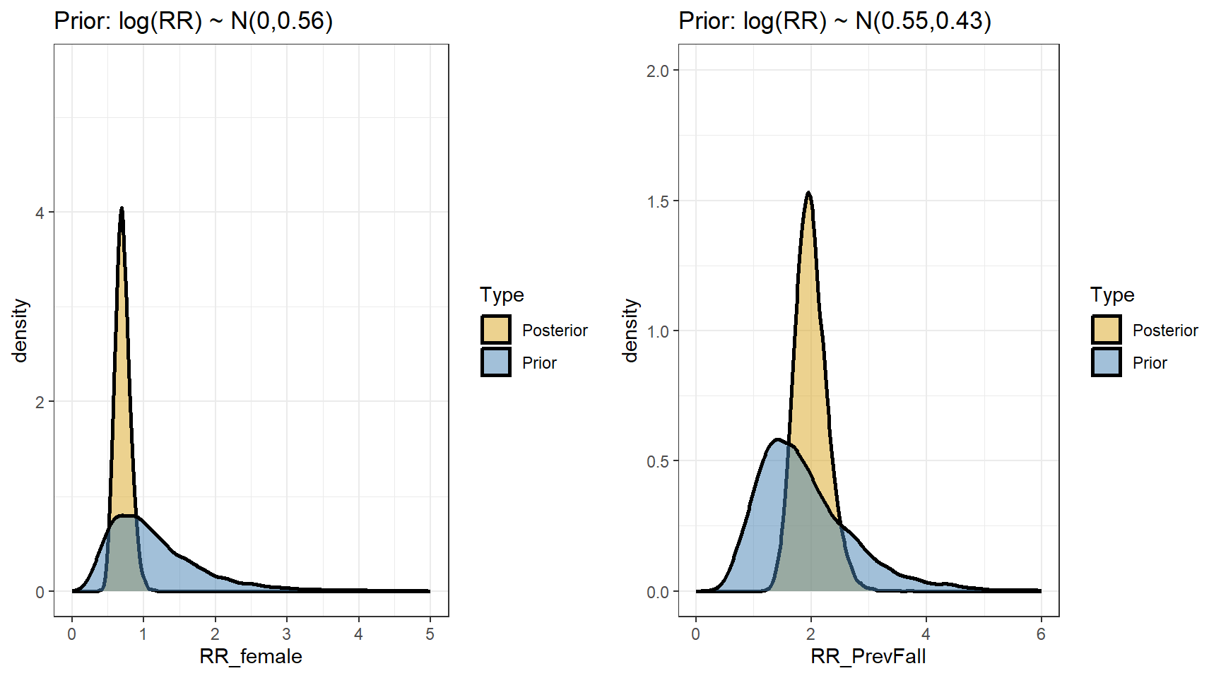
scale reduction factor on split chains (at convergence, Rhat = 1).

Comparing prior and posterior

Code

s1 <- posterior_samples(model1)
p1 <- data.frame(RR_female = c(exp(s1[,"b_FemaleSex"]),
                         exp(s1[,"prior_b_FemaleSex"])),
           Type=rep(c("Posterior","Prior"),
                    each=nrow(s1))) %>%
  ggplot(aes(x=RR_female,fill=Type))+
  geom_density(size=1,alpha=0.5)+
  xlim(c(0,3))+
  ylim(c(0,5.5))+
  labs(title="Prior: log(RR) ~ N(0,0.56)")+
  theme_bw()+
  scale_fill_manual(values=c("goldenrod","steelblue"))

p2 <-data.frame(RR_PrevFall = c(exp(s1[,"b_PrevFall"]),
                         exp(s1[,"prior_b_PrevFall"])),
           Type=rep(c("Posterior","Prior"),each=nrow(s1))) %>%
  ggplot(aes(x=RR_PrevFall,fill=Type))+
  geom_density(size=1,alpha=0.5)+
  xlim(c(0,5))+
  ylim(c(0,2))+
  labs(title="Prior: log(RR) ~ N(0.55,0.43)")+
  theme_bw()+
  scale_fill_manual(values=c("goldenrod","steelblue"))

ggarrange(p1,p2,nrow=1, ncol=2)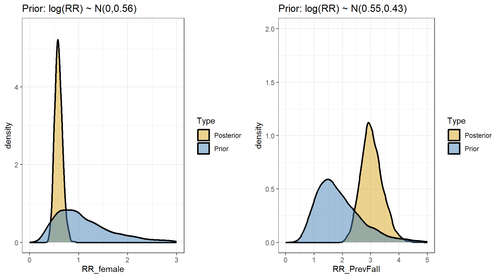

We are interested in computing the posterior distributions for the rate ratios

beta <- data.matrix(s1[,c("b_Intercept","b_FemaleSex","b_PrevFall")])

my.summary <- function(x){
  round(c(Mean=mean(x), Median=median(x), low=quantile(x,0.025), high=quantile(x, 0.975)),2)
}

t(apply(exp(beta),2,my.summary))

            Mean Median low.2.5% high.97.5%
b_Intercept 1.24   1.23     0.99       1.51
b_FemaleSex 0.59   0.59     0.45       0.76
b_PrevFall  3.04   3.01     2.36       3.86

suppose we are interested in predicting fall rates per year for the four types of subjects defined by sex and previous fall

# design matrix!
X<-cbind(MaleNoFall=c(1,0,0),
         FemaleNoFall=c(1,1,0),
         MalePrevFall=c(1,0,1),
         FemalePrevFall=c(1,1,1))
row.names(X) <- c("Intercept","Female","PrevFall")
X

          MaleNoFall FemaleNoFall MalePrevFall FemalePrevFall
Intercept          1            1            1              1
Female             0            1            0              1
PrevFall           0            0            1              1

Predictions <- exp(beta %*% X)
t(apply(Predictions,2,my.summary))

               Mean Median low.2.5% high.97.5%
MaleNoFall     1.24   1.23     0.99       1.51
FemaleNoFall   0.73   0.72     0.55       0.93
MalePrevFall   3.72   3.71     3.08       4.41
FemalePrevFall 2.18   2.17     1.69       2.74

Expanding the Poisson Model

The standard Poisson model says that the only random variation is due to the Poisson sampling
- i.e. all subjects with the same values of the predictors have the same rate
The variance is equal to the mean and with more predictors, the same issue holds

\[\log(\lambda_i) = \beta_0 + \sum \beta_j x_{ij}\] \[ Y_i \sim Pois(\lambda_i T_i)\]

All variability in the number of falls is either explained by the \(x_{ij}\) or Poisson variability (there is no separate variance parameter)
This may be insufficient:
- “Extra-Poisson” variability is common - variability in excess of what the Poisson allows.
- This could result from omission of important and unmeasured predictors of the rate
- Clustering, by doctor, hospital, practice could induce additional variation
- There may be real unexplainable random variation: \(\lambda_i\) is only the average rate for subjects with characteristics defined by the \(x_{ij}\)

Model 2. Expanding with Random Effect

As with the hospital mortality, seeds and RP models, we can include a random intercept for each individual
This allows that, on average, subjects with the same characteristics have the same rate
It also allows that some individuals have rates higher or lower than this
This mean that variation in the actual counts can be larger than their mean
The true log-rate for subject \(i\) is somewhere near

\[\log(\lambda_i) \approx \beta_0 + \sum \beta_j x_{ij}\]

Add normal random effects to the regression

\[\log(\lambda_i) \approx \beta_0 + \sum \beta_j x_{ij} + b_i\] \[ b_i \sim N(0, \sigma_b)\] \[ Y_i \sim Pois(\lambda_i T_i)\]

we can again examine the posterior distribution of \(\sigma_b\) to see if the random intercept added to the model is reasonable.
If \(\sigma_b\) is small, the Poisson distribution explains the between subject variability well enough

model2 <- brm(falls ~ FemaleSex + PrevFall + offset(log(fu)) + (1| Subject),
    data = dat, 
    family = "poisson",
    sample_prior=T,
    prior = c(prior(normal(0, 100), class = "Intercept"),
              prior(normal(0, 0.56), class = "b", coef=FemaleSex),
              prior(normal(0.55, 0.43), class = "b", coef=PrevFall)),
    chains = 4, 
    iter = 7500, 
    warmup = 5000, 
    cores = 4,
    seed = 123, 
    silent = 2,
    refresh = 0)

saveRDS(model2, "data/chap8_poisson_2")

Posterior summary

model2 <- readRDS("data/chap8_poisson_2")
plot(model2)

print(model2)

 Family: poisson 
  Links: mu = log 
Formula: falls ~ FemaleSex + PrevFall + offset(log(fu)) + (1 | Subject) 
   Data: dat (Number of observations: 162) 
  Draws: 4 chains, each with iter = 7500; warmup = 5000; thin = 1;
         total post-warmup draws = 10000

Multilevel Hyperparameters:
~Subject (Number of levels: 162) 
              Estimate Est.Error l-95% CI u-95% CI Rhat Bulk_ESS Tail_ESS
sd(Intercept)     1.48      0.17     1.18     1.83 1.00     3519     5707

Regression Coefficients:
          Estimate Est.Error l-95% CI u-95% CI Rhat Bulk_ESS Tail_ESS
Intercept    -0.78      0.26    -1.31    -0.31 1.00     7548     7477
FemaleSex    -0.46      0.28    -1.03     0.09 1.00     6873     7597
PrevFall      0.92      0.26     0.41     1.42 1.00     7213     7645

Draws were sampled using sampling(NUTS). For each parameter, Bulk_ESS
and Tail_ESS are effective sample size measures, and Rhat is the potential
scale reduction factor on split chains (at convergence, Rhat = 1).

Comparing prior and posterior

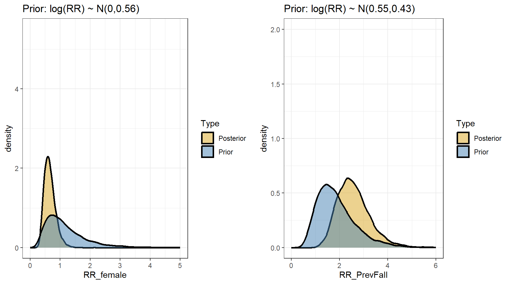
We are interested in computing the posterior distributions for the rate ratios

beta <- data.matrix(s2[,c("b_Intercept","b_FemaleSex","b_PrevFall")])
t(apply(exp(beta),2,my.summary))

            Mean Median low.2.5% high.97.5%
b_Intercept 0.47   0.46     0.27       0.74
b_FemaleSex 0.66   0.63     0.36       1.10
b_PrevFall  2.59   2.51     1.51       4.14

predicting the expected fall rates per year for the four types of subjects defined by sex and previous fall

# design matrix.
X<-cbind(MaleNoFall=c(1,0,0),
         FemaleNoFall=c(1,1,0),
         MalePrevFall=c(1,0,1),
         FemalePrevFall=c(1,1,1))
# row.names(X) <- c("Intercept","Female","PrevFall")
Predictions <- exp(beta %*% X)
t(apply(Predictions,2,my.summary))

               Mean Median low.2.5% high.97.5%
MaleNoFall     0.47   0.46     0.27       0.74
FemaleNoFall   0.30   0.29     0.16       0.49
MalePrevFall   1.19   1.15     0.65       1.89
FemalePrevFall 0.75   0.73     0.39       1.27

Model 3. Negative Binomial Model

A random variable Y is overdispersed if the observed variability in Y exceeds the variability expected by the assumed probability model of Y
Consider a negative regression model on \(Y\) with covariates \(X_1, \ldots, X_p\) and offset \(T\) (time), we have

\[ Y_i \mid \beta_0, \beta_1, \ldots, \beta_p, \mu_i, \gamma \sim NegBin(\mu_i, r)\]

\[ \log(\mu_i) = \beta_0 + \beta_1 X_{i1} + \ldots + \beta_p X_{ip}\]

The mean and variance are not equal! \[E(Y_i \mid \mu_i, \gamma) = \mu_i \text{ and } Var(Y_i \mid \mu_i, \gamma) = \mu_i + \frac{\mu_i^2}{\gamma}\]
Comparisons to the Poisson model
- For a large dispersion parameter \(\gamma\), \(E(Y)\approx Var(Y)\) and this model will approximate a Poisson model.
- For a small dispersion parameter \(\gamma\), \(E(Y) < Var(Y)\) and \(Y\) is overdispersed.

model3 <- brm(falls ~ FemaleSex + PrevFall + offset(log(fu)),
    data = dat, 
    family = "negbinomial",
    sample_prior=T,
    prior = c(prior(normal(0, 100), class = "Intercept"),
              prior(normal(0, 0.56), class = "b", coef=FemaleSex),
              prior(normal(0.55, 0.43), class = "b", coef=PrevFall)),
    chains = 4, 
    iter = 7500, 
    warmup = 5000, 
    cores = 4,
    seed = 123, 
    silent = 2,
    refresh = 0)

saveRDS(model3, "data/chap8_poisson_3")

Posterior summary

model3 <- readRDS("data/chap8_poisson_3")
plot(model3)

print(model3)

 Family: negbinomial 
  Links: mu = log; shape = identity 
Formula: falls ~ FemaleSex + PrevFall + offset(log(fu)) 
   Data: dat (Number of observations: 162) 
  Draws: 4 chains, each with iter = 7500; warmup = 5000; thin = 1;
         total post-warmup draws = 10000

Regression Coefficients:
          Estimate Est.Error l-95% CI u-95% CI Rhat Bulk_ESS Tail_ESS
Intercept     0.23      0.21    -0.18     0.65 1.00    11989     7562
FemaleSex    -0.37      0.27    -0.88     0.15 1.00    11723     7694
PrevFall      0.91      0.24     0.44     1.39 1.00    11545     8176

Further Distributional Parameters:
      Estimate Est.Error l-95% CI u-95% CI Rhat Bulk_ESS Tail_ESS
shape     0.39      0.08     0.26     0.56 1.00    12519     7943

Draws were sampled using sampling(NUTS). For each parameter, Bulk_ESS
and Tail_ESS are effective sample size measures, and Rhat is the potential
scale reduction factor on split chains (at convergence, Rhat = 1).

Comparing prior and posterior

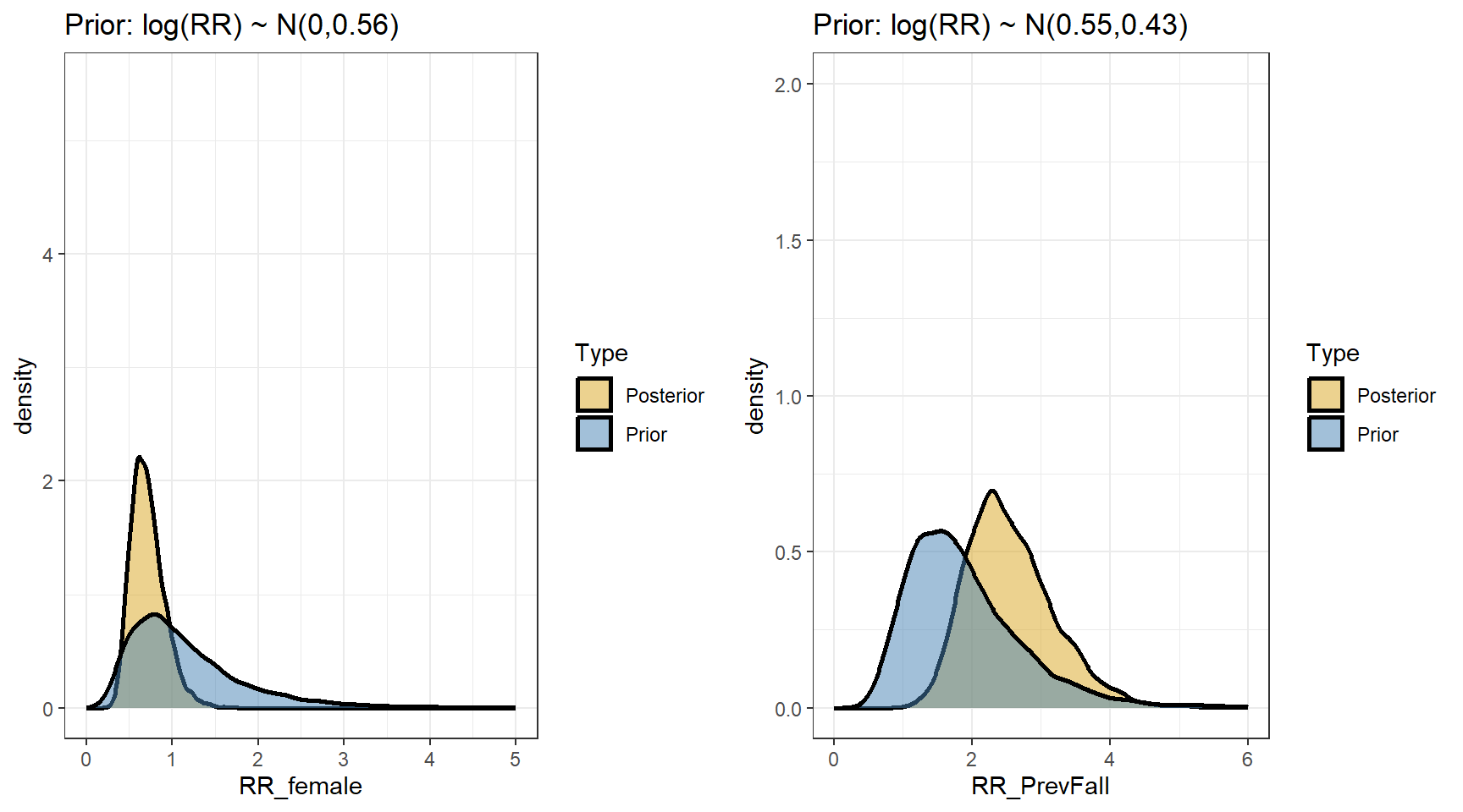
We are interested in computing the posterior distributions for the rate ratios

beta <- data.matrix(s3[,c("b_Intercept","b_FemaleSex","b_PrevFall")])
t(apply(exp(beta),2,my.summary))

            Mean Median low.2.5% high.97.5%
b_Intercept 1.28   1.25     0.83       1.91
b_FemaleSex 0.72   0.69     0.41       1.16
b_PrevFall  2.56   2.48     1.55       4.02

suppose we are interested in predicting fall rates per year for the four types of subjects defined by sex and previous fall

Predictions <- exp(beta %*% X)
t(apply(Predictions,2,my.summary))

               Mean Median low.2.5% high.97.5%
MaleNoFall     1.28   1.25     0.83       1.91
FemaleNoFall   0.89   0.87     0.55       1.39
MalePrevFall   3.19   3.10     2.02       4.89
FemalePrevFall 2.23   2.15     1.27       3.74

Model 4. Expanding with zero-inflation

Often, excessive numbers of zero counts are a problem (e.g., healthy individuals have no events and less healthy individuals can have many events)
The Poisson distribution with mean \(\theta\) has this probability of zero events:

\[P(Y=0 \mid \theta) = \frac{\theta^0 \exp(-\theta)}{0!} = \exp(-\theta)\]

e.g., if the mean is 5, \(P(Y=0) = 0.67\%\)
In a sample where a lot of people have high counts, so the mean is high, zeroes are unlikely
One solution is to fit a zero-inflated Poisson
It has two parts (“mixture model”)
- One regression fits a probability that \(\lambda_i = 0\) (explains some of the zeroes)
- A simultaneous regression fits the observed count (explains some of the zeroes)
The model says that some subjects have a true zero rate - one set of predictors is used for this
Among subjects with a non-zero rate, the observations are Poisson
To model this we need a new Bernoulli variable \(z\), \(z\) tells us which group (reg 1 for \(\lambda_i = 0\) or reg 2 for the observed counts) the observation is in: 0 or 1

\(z_i=1\) (\(Y_i = 0\), never have a fall during observation window, structural zeros)
\(z_i=0\) (\(Y_i > 0\), at least 1 a fall during observation window, structural non-zeros)

We are modelling the probability of seeing structural zeros (no falls/zero count) using a logistic regression adjusted for Previsou Falls.

\[Zero_i \sim dbern(p_i)\] \[logit(p_i) = \alpha_0 + \alpha_1 \times PrevFall_i\]

\(P(z_i=1)\) is the probability of zero count.
\(P(z_i=0) = 1 - P(z_i=1)\) is the probability of non-zero counts.

model4 <- brm(bf(falls ~ FemaleSex + PrevFall + offset(log(fu)),
                 zi ~ PrevFall), #being a non-faller
    data = dat, 
    family = zero_inflated_poisson(link_zi="logit"),,
    sample_prior=T,
    prior = c(prior(normal(0, 100), class = "Intercept"),
              prior(normal(0, 0.56), class = "b", coef=FemaleSex),
              prior(normal(0.55, 0.43), class = "b", coef=PrevFall)),
    chains = 4, 
    iter = 7500, 
    warmup = 5000, 
    cores = 4,
    seed = 123, 
    silent = 2,
    refresh = 0)

saveRDS(model4, "data/chap8_poisson_4")

Posterior summary

model4 <- readRDS("data/chap8_poisson_4")
plot(model4)

print(model4)

 Family: zero_inflated_poisson 
  Links: mu = log; zi = logit 
Formula: falls ~ FemaleSex + PrevFall + offset(log(fu)) 
         zi ~ PrevFall
   Data: dat (Number of observations: 162) 
  Draws: 4 chains, each with iter = 7500; warmup = 5000; thin = 1;
         total post-warmup draws = 10000

Regression Coefficients:
             Estimate Est.Error l-95% CI u-95% CI Rhat Bulk_ESS Tail_ESS
Intercept        1.00      0.12     0.76     1.23 1.00     9637     7576
zi_Intercept     0.34      0.23    -0.13     0.79 1.00    10325     7521
FemaleSex       -0.36      0.15    -0.65    -0.08 1.00    11138     7269
PrevFall         0.68      0.14     0.42     0.95 1.00     9183     7599
zi_PrevFall     -0.95      0.39    -1.72    -0.20 1.00    10259     7022

Draws were sampled using sampling(NUTS). For each parameter, Bulk_ESS
and Tail_ESS are effective sample size measures, and Rhat is the potential
scale reduction factor on split chains (at convergence, Rhat = 1).

Comparing prior and posterior

Computing the posterior distributions for the rate ratios

beta4 <- data.matrix(s4[,c("b_Intercept","b_FemaleSex","b_PrevFall","b_zi_PrevFall")])
t(apply(exp(beta4),2,my.summary))

              Mean Median low.2.5% high.97.5%
b_Intercept   2.73   2.72     2.14       3.41
b_FemaleSex   0.71   0.70     0.52       0.93
b_PrevFall    2.00   1.97     1.52       2.60
b_zi_PrevFall 0.42   0.39     0.18       0.82

Predicting fall rates per year for the four types of subjects defined by sex and previous fall

Z <- s4[,c("b_zi_Intercept","b_zi_PrevFall" )]
C <- s4[,c("b_Intercept","b_FemaleSex","b_PrevFall")]

# create a dataset with the 4 categories of patient and one year of follow-up
nd <- cbind(expand.grid(PrevFall=0:1,
                        FemaleSex=0:1),
            fu=1,
            Subject=999)

# probabilities of zero count for the falls and no-falls groups 
# irrespective of sex
# Pr0. is Pr(Z = 1 | PrevFall = 0), the probability of zero count for patients who had not fall previously;
Pr0. <- plogis(Z[,"b_zi_Intercept"])
# Pr1. is Pr(Z = 1 | PrevFall = 1), the probability of zero count for patients who had fall previously;
Pr1. <- plogis(Z[,"b_zi_Intercept"] + Z[,"b_zi_PrevFall"])

# (ij) = (prevfall, sex)
C00 <- exp(C[,"b_Intercept"])
C10 <- exp(C[,"b_Intercept"] + C[,"b_PrevFall"])
C01 <- exp(C[,"b_Intercept"] + C[,"b_FemaleSex"])
C11 <- exp(C[,"b_Intercept"] + C[,"b_FemaleSex"] + C[,"b_PrevFall"])

# probability of non-zero fall * mean rate of fall, if male and a previous non-faller
M00 <- (1-Pr0.) * C00  
# probability of non-zero fall * mean rate of fall, if male and a previous faller
M10 <- (1-Pr1.) * C10  
# probability of non-zero fall * mean rate of fall, if female and a previous non-faller
M01 <- (1-Pr0.)*C01 
# probability of non-zero fall * mean rate of fall, if female and a previous faller
M11 <- (1-Pr1.)*C11

# mean (expected) numbers of falls
round(rbind("No fall/male"=my.summary(M00),
      "Fall/male"=my.summary(M10),
      "No fall female"=my.summary(M01),
      "Fall/female"=my.summary(M11)),2)

               Mean Median low.2.5% high.97.5%
No fall/male   1.14   1.13     0.81       1.52
Fall/male      3.48   3.46     2.59       4.44
No fall female 0.80   0.79     0.55       1.10
Fall/female    2.44   2.42     1.73       3.31

Summarizing the observed rates by previous fall and sex from the data

group.by <- list(PrevFall=dat$PrevFall,
                 FemaleSex=dat$FemaleSex)

FU <- aggregate(x = dat$fu, group.by,  sum)
names(FU)[names(FU)=="x"] <- "FU"

FALLS <- aggregate(dat$falls,group.by,sum)
names(FALLS)[names(FALLS)=="x"] <- "Falls"

N <- aggregate(dat$falls,group.by,length)
names(N)[names(N)=="x"] <- "N"

temp <-   merge(FU,FALLS, 
                by=c("PrevFall","FemaleSex"))

falls.aggregate <- merge(temp,
                    N,
                  by=c("PrevFall","FemaleSex"))
falls.aggregate$Obs <- round(falls.aggregate$Falls/falls.aggregate$FU,2)

falls.aggregate %>%
  datatable(
  rownames = F,
  class = "compact",
  options = list(
    dom = 't',
    ordering = FALSE,
    paging = FALSE,
    searching = FALSE,
    columnDefs = list(list(className = 'dt-center', 
                      targets = 0:5))))

Combining results from all four models

Posterior summary

model	RR	mean	2.5%	97.5%
Poisson	female sex	0.59	0.45	0.76
	prev fall	3.01	2.37	3.86
Poisson/RE	female sex	0.63	0.36	1.09
	prev fall	2.53	1.52	4.20
NB	female sex	0.72	0.40	1.19
	prevfall	2.56	1.53	4.02
ZIP	RR:female sex	0.71	0.52	0.93
	RR:prev fall	2.00	1.51	2.61
	OR(zero):prev fall	0.42	0.18	0.83

Posterior predictive summary

PredictedRates <- cbind(
      Pois=predict(model1, newdata=nd)[,1],
      "P/RE"=predict(model2, newdata=nd, 
                        re_formula = ~1 | Subject, allow_new_levels=T)[,1],
      "NB"=predict(model3, newdata=nd)[,1],
      "ZIP"=predict(model4, newdata=nd)[,1])

PredictedRates <- cbind(nd[,1:2],round(PredictedRates,2))
PredictedRates <-merge(falls.aggregate[,c("N","Obs","PrevFall","FemaleSex")], 
      PredictedRates, by=c("PrevFall","FemaleSex"))

PredictedRates %>%
  datatable(
  rownames = F,
  class = "compact",
  options = list(
    dom = 't',
    ordering = FALSE,
    paging = FALSE,
    searching = FALSE,
    columnDefs = list(list(className = 'dt-center', 
                      targets = 0:7))))

Summary

RR are of similar size for each of the models
CrI are wider for all models that allow for extra-Poisson variation
In the ZIP model, being previous fall decreases the odds of being a non-faller (having a zero count)(OR=0.42)
- among the fallers, the effect of a previous fall (RR=2.0) is smaller than for the other models

Checking and comparing models

Dose simple Poisson fit the count outcome?

Comparing between the four models using loo

loo1 <- loo(model1)
loo2 <- loo(model2) #best model
loo3 <- loo(model3)
loo4 <- loo(model4)
loo_compare(loo1, loo2, loo3, loo4)

       elpd_diff se_diff
model2    0.0       0.0 
model3  -27.7       6.9 
model4 -126.5      53.3 
model1 -188.7      70.8

visually checking posterior predictive fits

p1<-pp_check(model1, ndraws = 50)
p2<-pp_check(model2, ndraws = 50)
p3<-pp_check(model3, ndraws = 50)
p4<-pp_check(model4, ndraws = 50)

ggarrange(p1,p2,p3,p4, nrow = 2, ncol=2)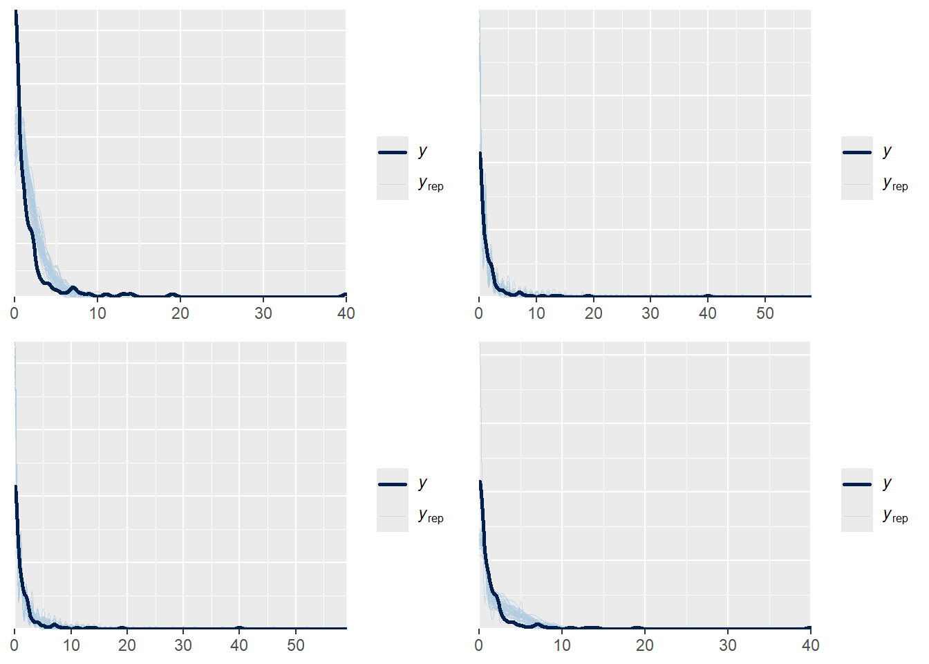

Poisson model fits worst and ZIP is the second worst
Poisson/RE fits the best, by a substantial margin

Examine dispersion

The Poisson random effects and negative binomial models have a parameter that measures extra-Poisson variability - In the Poisson/RE model, it is the standard deviation around the log-means
In the NB model, it is the standard deviation between the rates, based on the gamma distribution
Both model tell us over-dispersion exists in this data

#Poisson random effect model
model2

 Family: poisson 
  Links: mu = log 
Formula: falls ~ FemaleSex + PrevFall + offset(log(fu)) + (1 | Subject) 
   Data: dat (Number of observations: 162) 
  Draws: 4 chains, each with iter = 7500; warmup = 5000; thin = 1;
         total post-warmup draws = 10000

Multilevel Hyperparameters:
~Subject (Number of levels: 162) 
              Estimate Est.Error l-95% CI u-95% CI Rhat Bulk_ESS Tail_ESS
sd(Intercept)     1.48      0.17     1.18     1.83 1.00     3519     5707

Regression Coefficients:
          Estimate Est.Error l-95% CI u-95% CI Rhat Bulk_ESS Tail_ESS
Intercept    -0.78      0.26    -1.31    -0.31 1.00     7548     7477
FemaleSex    -0.46      0.28    -1.03     0.09 1.00     6873     7597
PrevFall      0.92      0.26     0.41     1.42 1.00     7213     7645

Draws were sampled using sampling(NUTS). For each parameter, Bulk_ESS
and Tail_ESS are effective sample size measures, and Rhat is the potential
scale reduction factor on split chains (at convergence, Rhat = 1).

model3

 Family: negbinomial 
  Links: mu = log; shape = identity 
Formula: falls ~ FemaleSex + PrevFall + offset(log(fu)) 
   Data: dat (Number of observations: 162) 
  Draws: 4 chains, each with iter = 7500; warmup = 5000; thin = 1;
         total post-warmup draws = 10000

Regression Coefficients:
          Estimate Est.Error l-95% CI u-95% CI Rhat Bulk_ESS Tail_ESS
Intercept     0.23      0.21    -0.18     0.65 1.00    11989     7562
FemaleSex    -0.37      0.27    -0.88     0.15 1.00    11723     7694
PrevFall      0.91      0.24     0.44     1.39 1.00    11545     8176

Further Distributional Parameters:
      Estimate Est.Error l-95% CI u-95% CI Rhat Bulk_ESS Tail_ESS
shape     0.39      0.08     0.26     0.56 1.00    12519     7943

Draws were sampled using sampling(NUTS). For each parameter, Bulk_ESS
and Tail_ESS are effective sample size measures, and Rhat is the potential
scale reduction factor on split chains (at convergence, Rhat = 1).

Conclusions

The likelihood and starting point for modelling count data is usually the Poisson
It is often the case that the Poisson is too simple - can’t account for all the variability in counts
Negative binomial and normal random effects models allow additional variation in rates
ZIP models allow an excess of zeroes, possibly dependent on predictors
ZI NB models are also possible
Check model fits (wait, loo - can be technical problems with these)

References

Cook, Wendy L, George Tomlinson, Meghan Donaldson, Samuel N Markowitz, Gary Naglie, Boris Sobolev, and Sarbjit V Jassal. 2006. “Falls and Fall-Related Injuries in Older Dialysis Patients.” Clinical Journal of the American Society of Nephrology 1 (6): 1197–1204.