Estimate and interpret algorithmic fairness metrics from a Bayesian logistic regression model
Conduct Bayesian meta-regression for binary outcomes
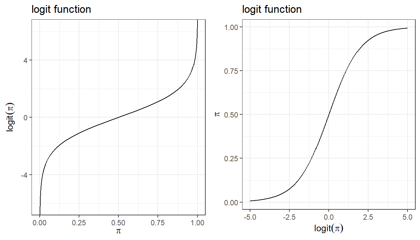
1. Logistic regression
1.1 Models for Binary Data
For binary outcome Y, we are interested to model the probability of \(\pi_i = P(Y_i=1)\), \(i=1, \ldots, n\)
\[Y_i \mid \pi_i, n_i \sim Bern(\pi_i)\]
\[ E(Y_i \mid \pi_i) = \pi\]
\[logit( \pi_i) = \beta_0 + \beta_1 X_{i1}\]
logistic regression model featuring logit link that connects binary outcome to a conventional linear regression format, is part of the broader class of generalized linear models
Independent observations. This assumption can be modified if working with clustered data.
Linear relationship between continuous covariates and log-odds We can check this assumption by examining marginal plots comparing the model predicted relationship between outcome (log-odds or logit-probability) and each continuous covariates.
Multicollinearity Multicollinearity is the phenomenon when a number of the explanatory variables are strongly correlated.
Correctly specified regression model This means that all relevant predictors for the response variable have been included in the model. This is often difficult to verify, but we can use posterior predictive distribution to check for regression fit. We can also use WAIC and LOO to compare different models.
Comparing to linear regression model we no-longer require the residuals to be normally distributed and homoscedasticity.
1.3 Working example: diagnostic Sensitivity analysis
Each study reports observed positive chemiluminescent immunoassa (CLIA, \(r_i\)) and number having positive reference standard reverse transcriptase polymerase chain reaction (RT-PCR, \(n_i\))
Interest lies in summarizing this collection of values
 Family: binomial
  Links: mu = logit
Formula: r | trials(n) ~ 1
   Data: dat (Number of observations: 10)
  Draws: 4 chains, each with iter = 2000; warmup = 1000; thin = 1;
         total post-warmup draws = 4000

Population-Level Effects:
          Estimate Est.Error l-95% CI u-95% CI Rhat Bulk_ESS Tail_ESS
Intercept     1.33      0.06     1.21     1.46 1.01     1425     1875

Draws were sampled using sampling(NUTS). For each parameter, Bulk_ESS
and Tail_ESS are effective sample size measures, and Rhat is the potential
scale reduction factor on split chains (at convergence, Rhat = 1).
Model 2. Unpooled model with non-informative prior
fit3 <-brm(r |trials(n) ~1+(1|Study),data = dat,prior =c(prior(normal(0, 5), class = Intercept),prior(student_t(3, 0, 10), class = sd)),family = binomial,seed =123)saveRDS(fit3, "data/chp5_binary3")
fit3 <-readRDS("data/chp5_binary3")print(fit3)
 Family: binomial
  Links: mu = logit
Formula: r | trials(n) ~ 1 + (1 | Study)
   Data: dat (Number of observations: 10)
  Draws: 4 chains, each with iter = 2000; warmup = 1000; thin = 1;
         total post-warmup draws = 4000

Group-Level Effects:
~Study (Number of levels: 10)
              Estimate Est.Error l-95% CI u-95% CI Rhat Bulk_ESS Tail_ESS
sd(Intercept)     1.38      0.45     0.77     2.47 1.00      725     1311

Population-Level Effects:
          Estimate Est.Error l-95% CI u-95% CI Rhat Bulk_ESS Tail_ESS
Intercept     1.62      0.45     0.74     2.59 1.01      698     1030

Draws were sampled using sampling(NUTS). For each parameter, Bulk_ESS
and Tail_ESS are effective sample size measures, and Rhat is the potential
scale reduction factor on split chains (at convergence, Rhat = 1).
# define expit function; # transform model estimated log odds to probability scale;expit <-function(x){exp(x)/(1+exp(x))}## 1. Create one row per Study with n = 1 so that## the expected number of successes equals the success-probabilitynewdat <- dat %>%distinct(Study) %>%mutate(n =1) # one Bernoulli trial# 2. Draw posterior expectations that INCLUDE the random interceptdraws <-posterior_epred( fit3,newdata = newdat,re_formula =NULL# keep group-level effects) # summarize posterior probability;prob_summaries <-t(apply(draws, 2, quantile, probs =c(.025, .5, .975))) %>%as.data.frame() %>%setNames(c("median", "lower_95", "upper_95")) %>%mutate(Study = newdat$Study)prob_summaries
      median  lower_95  upper_95     Study
1  0.7372276 0.8262236 0.8970372       Lin
2  0.9338387 0.9640941 0.9834530        Ma
3  0.5183541 0.5753933 0.6332119       Cai
4  0.6106512 0.7307572 0.8314371 Infantino
5  0.8869331 0.9625789 0.9934809     Zhong
6  0.3354143 0.5192255 0.6983388       Jin
7  0.7578684 0.9154367 0.9854626       Xie
8  0.6438882 0.7064076 0.7646523  Yangchun
9  0.8266485 0.8589106 0.8881886      Qian
10 0.7807128 0.8639924 0.9254228       Lou
both model 2 and model 3 fit the data well. There is no substantial difference in model fit using LOO between model 2 and 3. If we are to select the best model, we will proceed with model 3.
Generalized linear models
We can specify the type of model by two features - Family: type of outcome (binomial, normal, Poisson, gamma) - Link: relationship between mean parameter and predictor (identity, logic, log)
computing posterior predicted probability of event (in this case the sensitivity of the CLIA test)
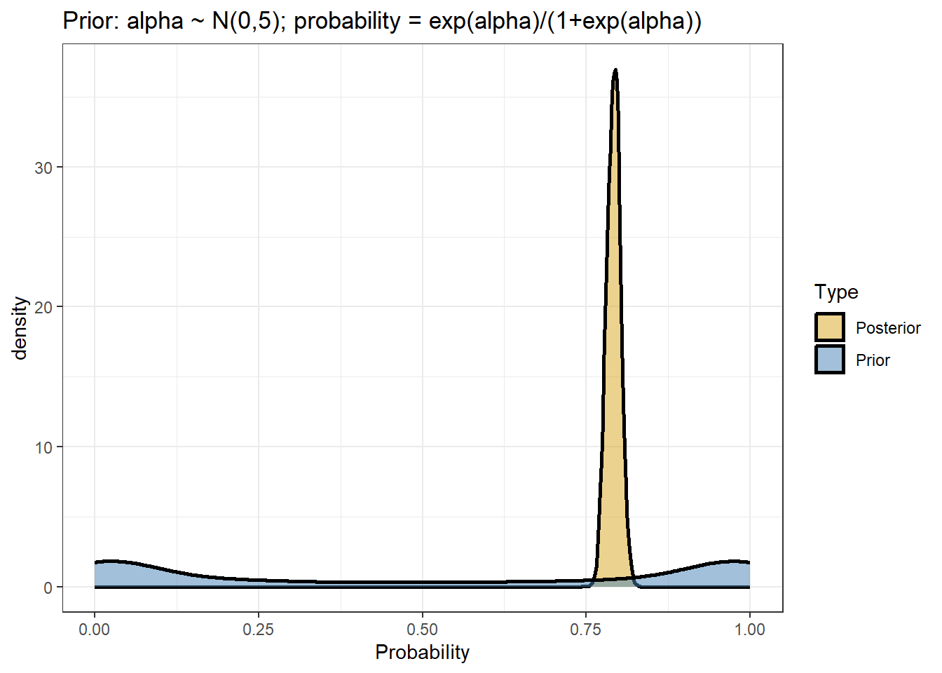
#posterior draws of log-odds estimate - the intercept;posterior <-posterior_samples(fit1)#posterior predicted probability of event;prob.pooled <-expit(posterior$b_Intercept)mean(prob.pooled)
[1] 0.7914033
quantile(prob.pooled, c(0.025, 0.975))
     2.5%     97.5%
0.7711078 0.8119101
comparing prior and posterior distribution visually
data.frame(Probability =c(inv_logit_scaled(posterior[,"b_Intercept"]),inv_logit_scaled(posterior[,"prior_Intercept"])),Type=rep(c("Posterior","Prior"),each=nrow(posterior))) %>%ggplot(aes(x=Probability,fill=Type))+geom_density(size=1,alpha=0.5)+labs(title="Prior: alpha ~ N(0,5); probability = exp(alpha)/(1+exp(alpha))")+theme_bw()+scale_fill_manual(values=c("goldenrod","steelblue"))
2. Logistic regression with predictors
Adding one predictor, age, for each study in modelling CLIA sensitivity
computing posterior predicted probability of event (in this case the sensitivity of the CLIA test)
fit4 <-readRDS("data/chp5_binary4")#posterior draws of log-odds estimate - the intercept;posterior <-posterior_samples(fit4)# beta posterior summaryexp(mean(posterior$b_age))
[1] 1.070023
exp(quantile(posterior$b_age, c(0.025, 0.975)))
    2.5%    97.5%
1.057597 1.083063
#posterior predicted probability testing positive for each study;pp<-posterior_predict(fit4)mean.pp<-colMeans(pp)/dat$nlci.pp<-apply(pp, 2, function(x) quantile(x, 0.025))/dat$nuci.pp<-apply(pp, 2, function(x) quantile(x, 0.975))/dat$npp.table <-data.frame(Study = dat$Study, r = dat$r, n = dat$n,Prob_obs =round(dat$r/dat$n,2),Prob_post =round(mean.pp,2),CI_post =paste0("(",round(lci.pp,2),",",round(uci.pp,2),")"))pp.table %>%datatable(rownames = F,class ="compact",options =list(dom ='t',ordering =FALSE,paging =FALSE,searching =FALSE,columnDefs =list(list(className ='dt-center', targets =0:5))))
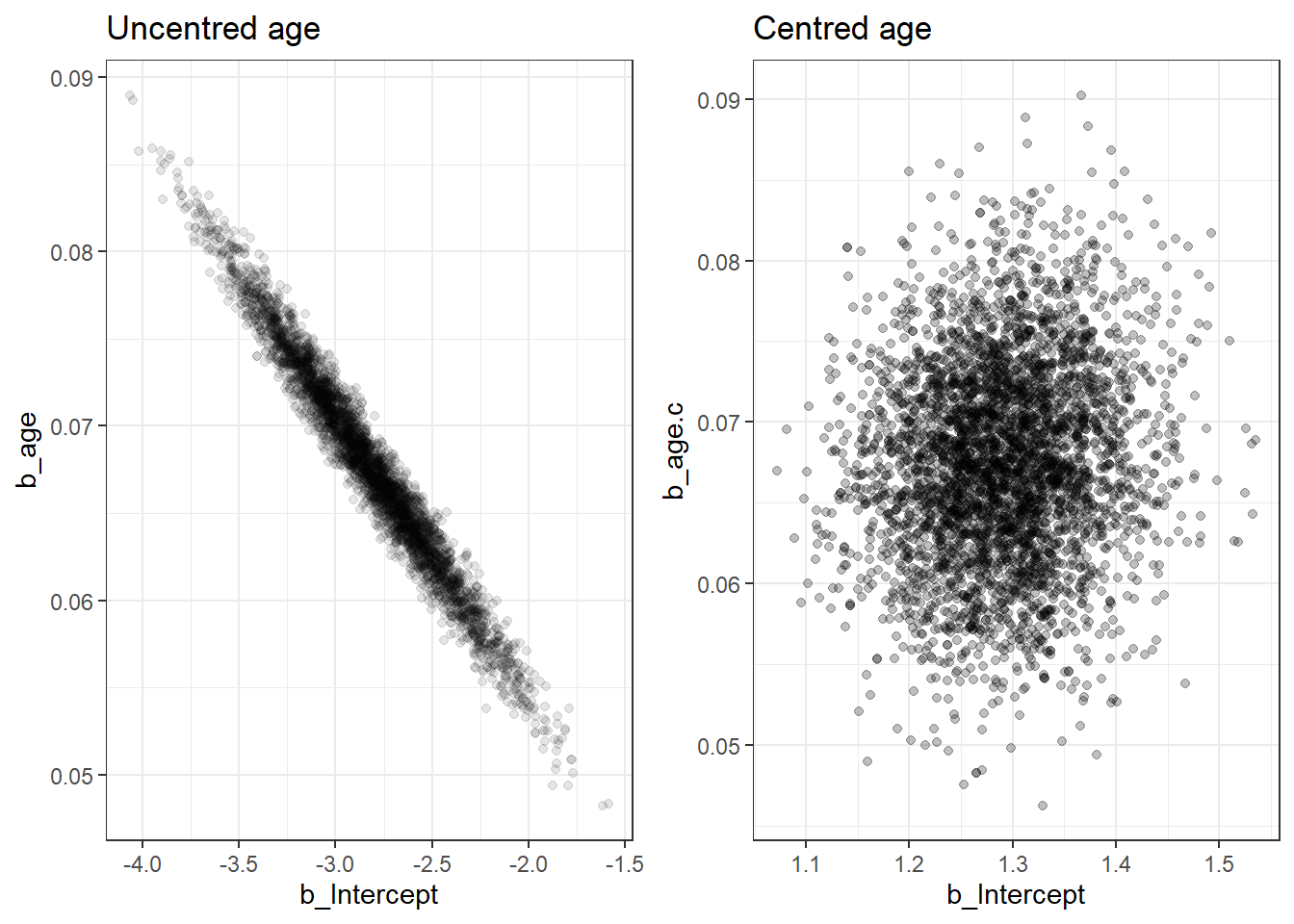
2.1 Centring continuous variable
our model says that sensitivity is different across studies according to the average age
Using a centred predictor also reduces correlation between intercept and slope. This can speed up MCMC convergence in some models (computationally more efficient).
comparing posterior distribution between centred and uncentred models
fit4c <-readRDS("data/chp5_binary4c")#posterior draws of log-odds estimate - the intercept;posteriorc <-posterior_samples(fit4c)# beta posterior summaryexp(mean(posteriorc$b_age))
[1] 1.069927
exp(quantile(posteriorc$b_age, c(0.025, 0.975)))
    2.5%    97.5%
1.057407 1.082997
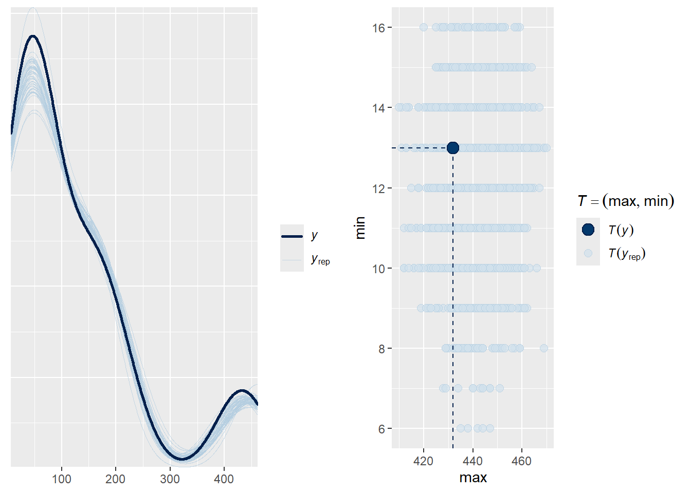
posterior predicted probability testing positive for each study comparing between the centred and uncentred models
we can see the results are almost identical and we achieved this with only 5000 iterations for the centred model.
We can investigate the correlation between two posterior regression parameters, \(\alpha\) (intercept) and \(\beta\) (log-OR for age).
The two parameters should be uncorrelated by model assumption! If you see visible correlation, you can consider thinning your MCMC or run more iterations.
p1<-pp_check(fit4c, ndraws =50)p2<-pp_check(fit4c, type ="stat_2d", stat =c("max", "min"))ggarrange(p1,p2, nrow =1)
3 Additional topics on Bayesian logistic regression models
In this example, we will conduct an analysis using a Bayesian logistic regression model.
Data come from a cross-sectional study of 1,225 smokers over the age of 40.
Each participant was assessed for chronic obstructive pulmonary disease (COPD), and characteristics of the type of cigarette they most frequently smoke were recorded.
The objective of the study was to identify associations between COPD diagnosis and cigarette characteristics
We will use the following variables from this data set:
TYPE: Type of cigarette, 1 = Menthol, 0 = Regular
NIC: Nicotine content, in mg
TAR: Tar content, in mg
LEN: Length of cigarette, in mm
FLTR: 1 = Filter, 0 = No Vlter
copd: 1 = COPD diagnosis, 0 = no COPD diagnosis
We fit a simple logistic regression, predicting the risk of Copd by Type of cigarette, Nicotine content, and Filter status.
We specify uninformative prior on log.odds, \(N(0,10)\)
m1_bern <-brm(copd ~ TYPE + NIC + FLTR, data = copd, family =bernoulli(link ="logit"), prior =c(prior(normal(0,10), class ="b"), prior(normal(0,10), class ="Intercept")),seed =123, silent =2, refresh =0)saveRDS(m1_bern, file="data/chp6_logistic")
 Family: bernoulli
  Links: mu = logit
Formula: copd ~ TYPE + NIC + FLTR
   Data: copd (Number of observations: 1225)
  Draws: 4 chains, each with iter = 2000; warmup = 1000; thin = 1;
         total post-warmup draws = 4000

Population-Level Effects:
          Estimate Est.Error l-95% CI u-95% CI Rhat Bulk_ESS Tail_ESS
Intercept    -2.94      0.64    -4.20    -1.71 1.00     3108     2483
TYPE          0.25      0.21    -0.19     0.66 1.00     3480     2501
NIC           1.30      0.35     0.61     1.99 1.00     3306     2723
FLTR         -0.60      0.44    -1.42     0.29 1.00     3344     2878

Draws were sampled using sampling(NUTS). For each parameter, Bulk_ESS
and Tail_ESS are effective sample size measures, and Rhat is the potential
scale reduction factor on split chains (at convergence, Rhat = 1).
# Directly from the posterior of exp(beta):draws_beta_TYPE <-as.matrix(m1_bern, pars ="b_TYPE")exp_beta_TYPE <-exp(draws_beta_TYPE)quantile(exp_beta_TYPE, probs =c(.025, 0.5, .975))
     2.5%       50%     97.5%
0.8286483 1.2832394 1.9293951
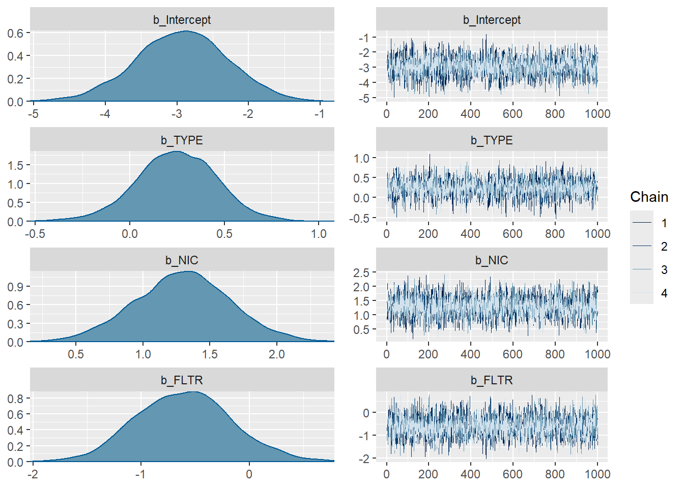
plot(m1_bern)
Posterior Distribution + Trace plot combining all chains
Good mixing from trace plot
Rhats’ are all less then 1.01, convergence!
Other diagnostic plots below
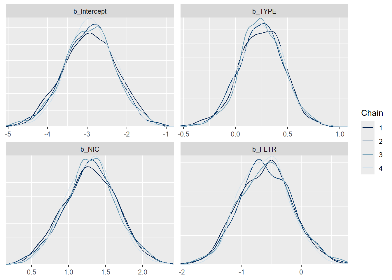
mcmc_dens_overlay(m1_bern, pars =c("b_Intercept", "b_TYPE", "b_NIC", "b_FLTR"))
Posterior density plot by chain
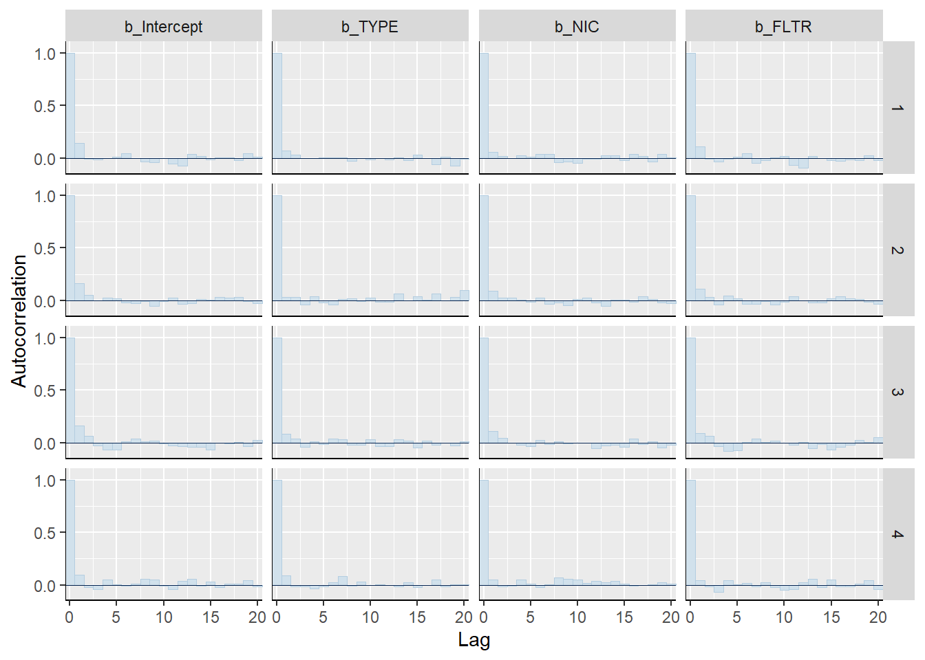
mcmc_acf_bar(m1_bern, pars =c("b_Intercept", "b_TYPE", "b_NIC", "b_FLTR"))
Posterior density plot by chain
3.1 Regression regularization and shrinkage priors
When the number of parameters to be estimated is large relative to sample size, estimation using non-informative or weakly informative priors tend to overfit.
One way to avoid overfitting is to perform regularization, that is, to shrink some of the parameters to closer to zero. This makes the model fit less well to the existing data, but will be much more generalizable to an independent data set.
Sparsity-Inducing Priors
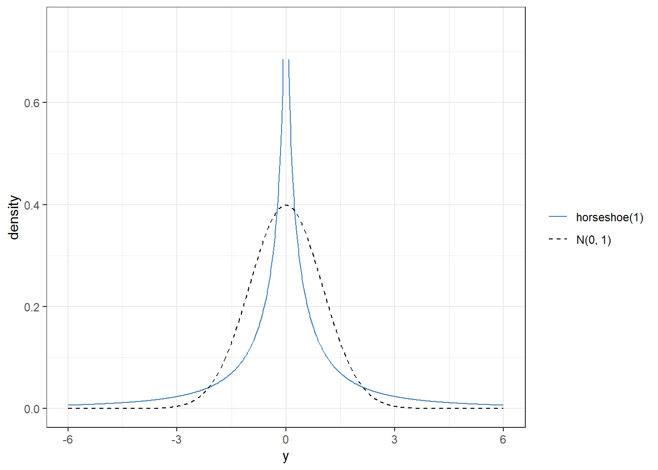
The horseshoe prior is a type of hierarchical prior for regression models by introducing a global scale and local scale parameters on the priors for the regression coefficients.
4. Bayesian Variable Selection for Logistic Regression
4.1 Why variable selection matters in logistic regression
In clinical and epidemiological research, we often have many candidate predictors, but only a subset are meaningfully associated with the outcome. The challenges for logistic regression in particular are:
Binary outcomes carry less information per observation than continuous ones, so overfitting is more likely with many predictors.
Standard non-informative priors do not prevent the model from assigning non-negligible probability mass to implausibly large log-odds ratios for noise predictors.
We want a model that is both interpretable and predictively sharp.
Two complementary Bayesian strategies are:
Shrinkage priors (horseshoe) - fit all variables simultaneously and let the prior pull small effects toward zero.
Projection predictive variable selection (projpred) - start from a well-regularized reference model and find the minimal subset of predictors that preserves its predictive performance.
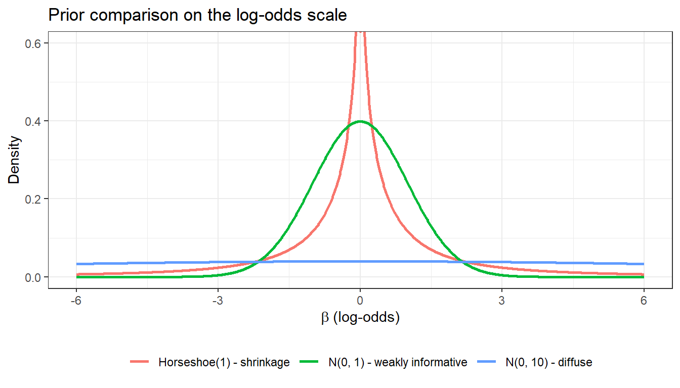
4.2 Prior visualization for shrinkage on the log-odds scale
Before fitting, it is good practice to visualize what your shrinkage prior implies for the regression coefficients. A \(N(0, 10)\) prior places substantial mass far beyond that range and provides little regularization. The horseshoe prior, by contrast, keeps most mass near zero while retaining heavy tails.
For most applied logistic regression analyses, \(N(0, 2.5)\) for slopes (Gelman recommendation) or the horseshoe are sensible defaults when variable selection is the goal.
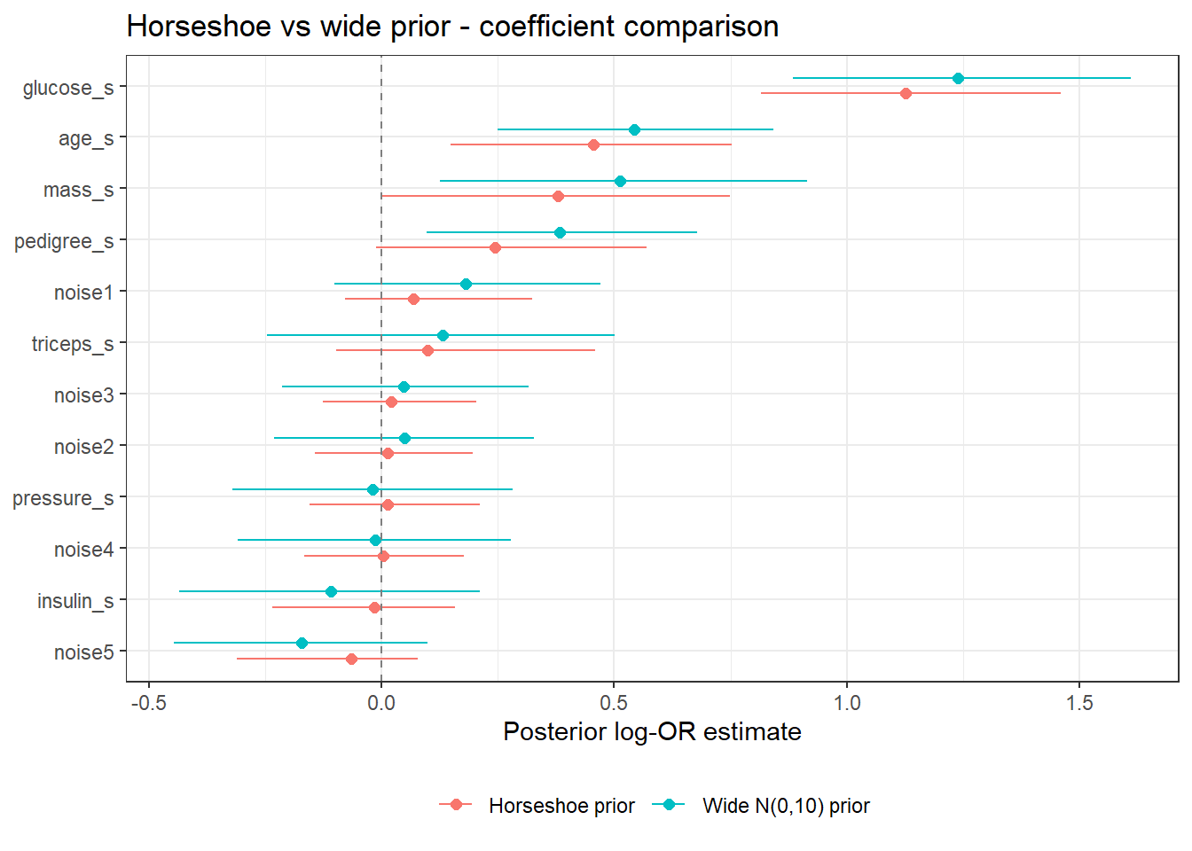
4.3 Simulate a logistic data set with many predictors
We use the mlbench package’s Pima Indians diabetes data, augmented with noise predictors, to illustrate variable selection.
Notice how the horseshoe shrinks the noise predictors aggressively toward zero, while the wide prior leaves them spread out.
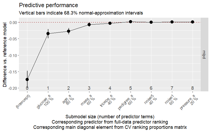
4.6 Projection predictive variable selection
The projpred package (Piironen et al. 2025) takes the full horseshoe posterior as a reference model and finds the minimal variable subset that preserves predictive performance. This avoids re-fitting many sub-models and propagates posterior uncertainty correctly.
library(projpred)# Step 1: build the reference model objectrefm_logistic <-get_refmodel(fit_hs_logistic)# Step 2: cross-validated variable selection# (set eval=FALSE in class; run once and save)# cv_fits_logistic <- run_cvfun(refm_logistic, k = 5)# cvvs_logistic <- cv_varsel(# refm_logistic,# cv_method = "kfold",# cvfits = cv_fits_logistic,# method = "L1",# nterms_max = 8,# verbose = 0# )# saveRDS(cvvs_logistic, "data/chp8_cvvs_logistic")# cvvs_logistic <- readRDS("data/chp8_cvvs_logistic")# Step 3: plot ELPD by model size# png("data/chp8_cvvs_mlpd.png", width = 800, height = 500, res = 120)# options(projpred.plot_vsel_show_cv_proportions = TRUE)# plot(cvvs_logistic, stats = "mlpd", deltas = TRUE)# dev.off()# Save suggested size and ranking as RDS (tiny objects)# saveRDS(suggest_size(cvvs_logistic, stat = "mlpd"), "data/chp8_suggest_size.rds")# saveRDS(ranking(cvvs_logistic), "data/chp8_ranking.rds")# Load pre-saved outputs - no need to load cvvs_logisticknitr::include_graphics("data/chp8_cvvs_mlpd.png")
The plot shows how much predictive performance (in mean log predictive density, MLPD) is lost as we remove predictors one by one. A model is considered adequate when the MLPD is within one standard error of the full reference model. suggest_size() returns the smallest model satisfying this criterion.
4.7 Posterior inclusion probabilities via hypothesis()
As a complementary summary, we can use hypothesis() to compute the posterior probability that each log-OR exceeds zero (i.e., a positive effect):
# Get all b_ parameters except interceptparam_names <-variables(fit_hs_logistic)param_names <- param_names[grepl("^b_", param_names)]param_names <- param_names[!grepl("Intercept", param_names)]# Strip the b_ prefix for hypothesis()param_names_clean <-gsub("^b_", "", param_names)# Wrap in backticks to handle any special charactersh_pos <-paste0("`", param_names_clean, "` > 0")hyp_out <-hypothesis(fit_hs_logistic, h_pos)hyp_out$hypothesis %>%arrange(desc(Post.Prob)) %>%mutate(across(where(is.numeric), \(x) round(x, 3))) %>%datatable(rownames =FALSE,options =list(dom ='t', pageLength =15,columnDefs =list(list(className ='dt-center', targets =0:5))))
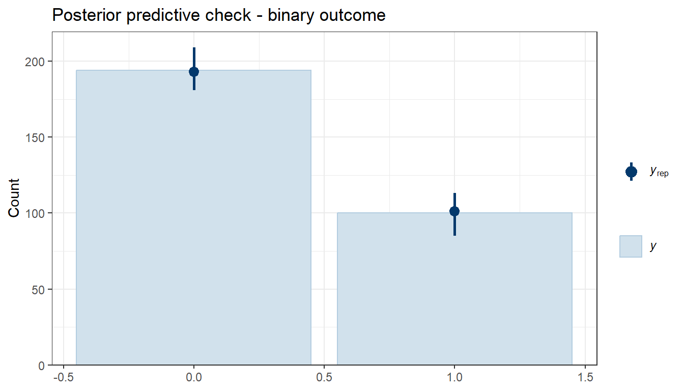
Fitting a logistic regression model to estimate associations is not the same as building a predictive model. When the goal is prediction, we care about:
Discrimination: can the model rank high-risk individuals above low-risk ones? (AUC / c-statistic)
Calibration: do predicted probabilities agree with observed event rates?
Overall accuracy: what is the average prediction error? (Brier score)
In the Bayesian framework, each of these metrics is computed from the posterior predictive distribution, so we obtain a full uncertainty distribution over each metric - not just a point estimate.
5.2 Working data: Pima Indians diabetes (complete cases)
We continue with the pima dataset from Section 4. We split into training and test sets to evaluate out-of-sample performance.
set.seed(2024)n_total <-nrow(pima)train_id <-sample(seq_len(n_total), size =floor(0.75* n_total))pima_train <- pima[train_id, ]pima_test <- pima[-train_id, ]cat("Training n =", nrow(pima_train), "| Test n =", nrow(pima_test), "\n")
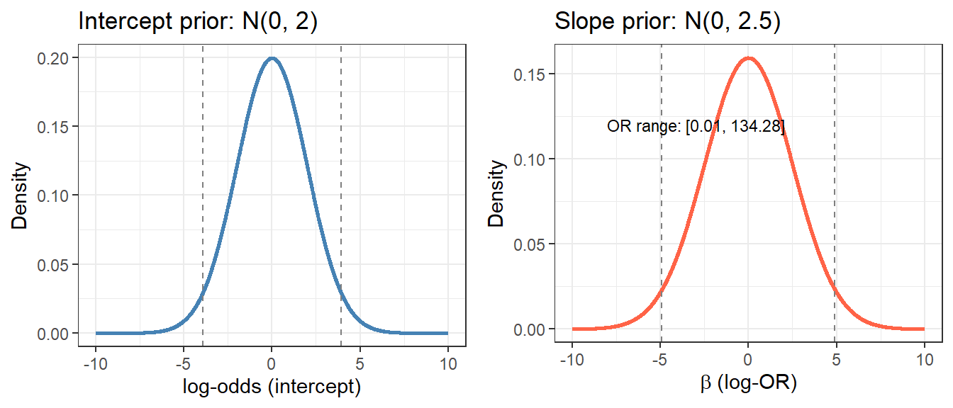
We use weakly informative priors. For standardized predictors, \(N(0, 2.5)\) on slopes means that a one-SD change in a predictor shifts log-odds by at most \(\pm 5\) units in 95% of the prior - already quite permissive.
5.6 Extract posterior predicted probabilities on the test set
# epred gives E[Y | X, theta] integrated over posterior = P(Y=1 | X)pred_draws <-posterior_epred( fit_pred,newdata = pima_test,allow_new_levels =TRUE)# dim: (n_draws x n_test)# Posterior mean predicted probability for each test observationp_hat <-colMeans(pred_draws) # posterior meanpima_test <- pima_test %>%mutate(p_hat = p_hat)
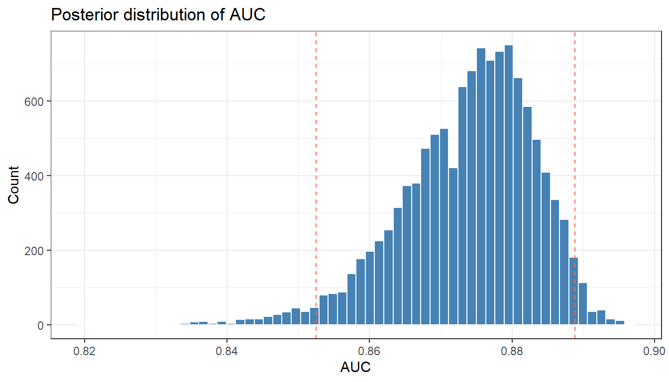
5.7 Discrimination: AUC / c-statistic
The AUC summarizes the probability that the model assigns a higher predicted risk to a randomly chosen case than to a randomly chosen non-case.
library(pROC)roc_obj <-roc(pima_test$diabetes_bin, pima_test$p_hat,quiet =TRUE)# Point estimate AUC using posterior mean probabilitiesauc_point <-auc(roc_obj)cat("AUC (posterior mean predictions):", round(auc_point, 3), "\n")
AUC (posterior mean predictions): 0.881
# Bayesian uncertainty in AUC: compute AUC for each posterior drawauc_draws <-apply(pred_draws, 1, function(p) {tryCatch(as.numeric(auc(roc(pima_test$diabetes_bin, p, quiet =TRUE))),error =function(e) NA_real_ )})auc_df <-tibble(auc = auc_draws[!is.na(auc_draws)])ggplot(auc_df, aes(x = auc)) +geom_histogram(bins =60, fill ="steelblue", colour ="white") +geom_vline(xintercept =quantile(auc_df$auc, c(0.025, 0.975)),linetype ="dashed", colour ="tomato") +labs(title ="Posterior distribution of AUC",x ="AUC", y ="Count") +theme_bw()
quantile(auc_df$auc, c(0.025, 0.5, 0.975))
     2.5%       50%     97.5%
0.8524590 0.8750554 0.8887904
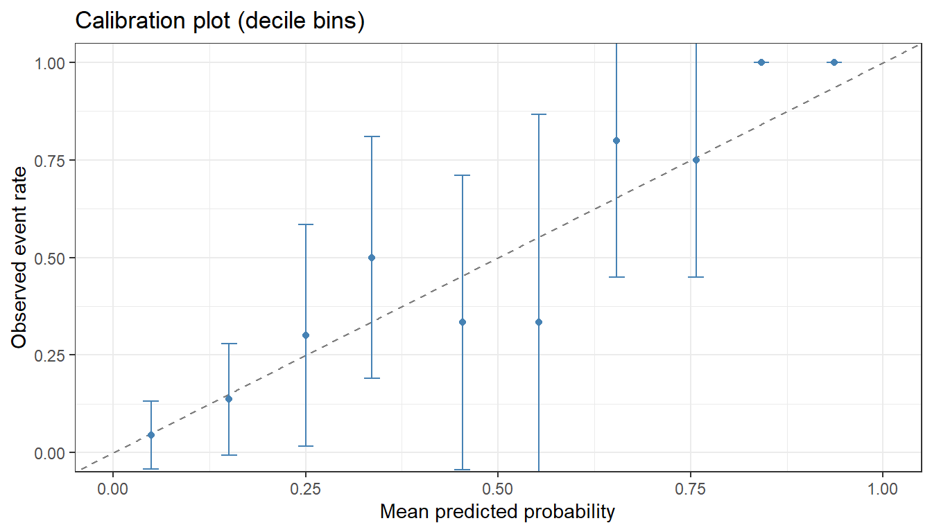
5.8 Calibration
Calibration assesses whether predicted probabilities match observed event rates. We use a calibration plot (decile bins) and the Expected Calibration Error (ECE).
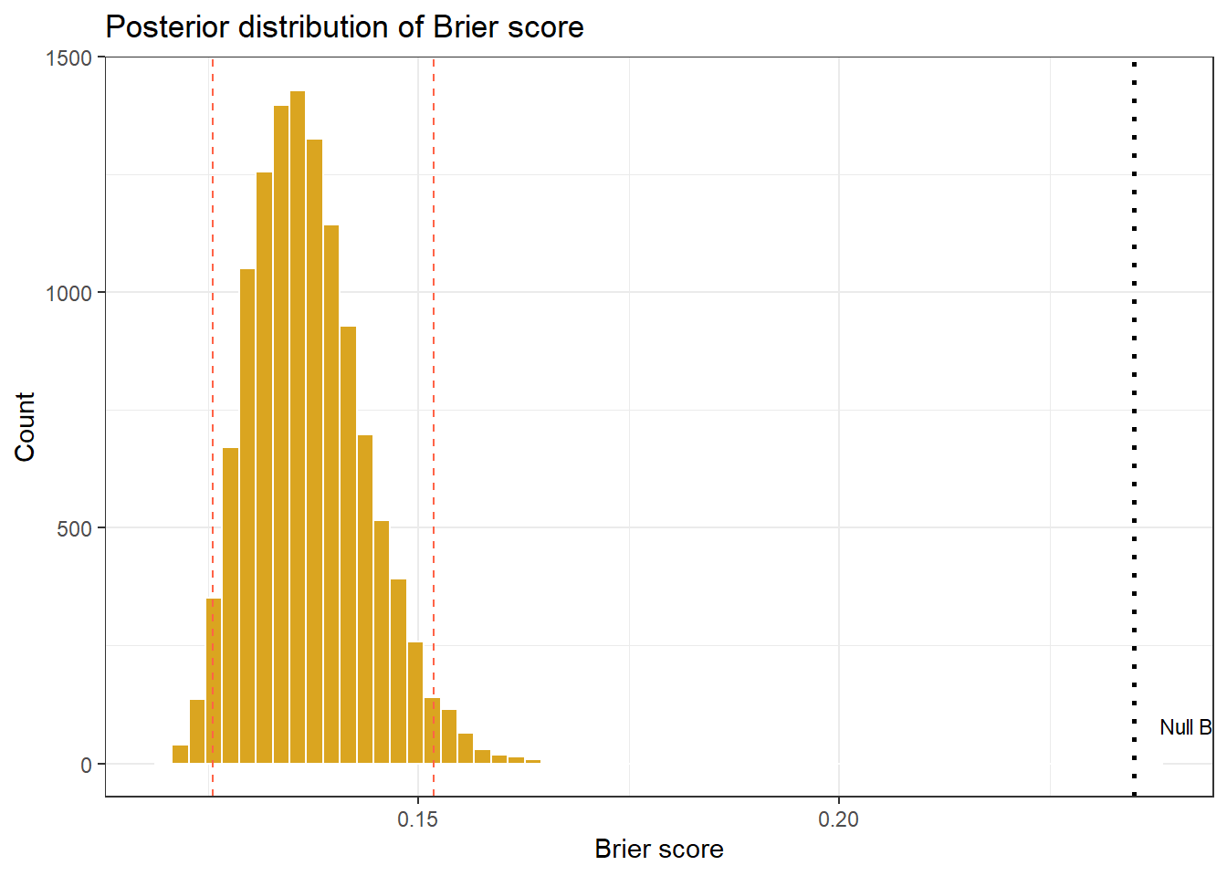
The Brier score is the mean squared error between predicted probabilities and observed binary outcomes. Lower is better; a model predicting the prevalence everywhere has a Brier score equal to \(p(1-p)\).
6. Bayesian Fairness Analysis for Logistic Regression
6.1 What is algorithmic fairness?
When logistic regression models inform decisions (e.g., screening, treatment allocation, risk stratification), we should check whether the model performs equally well across demographic subgroups. Algorithmic fairness asks: does the model disadvantage any group relative to another?
There is no single universally agreed definition of fairness. Key metrics capture different normative perspectives and - importantly - they cannot all be satisfied simultaneously when base rates differ across groups (the “impossibility theorems”).
6.2 Fairness metrics: definitions
Let \(A \in \{0, 1\}\) be a protected attribute (e.g., Sex: 0 = female, 1 = male), \(\hat{Y}\) be the model’s prediction (binary, based on a threshold \(\tau\)), and \(Y\) the true outcome.
Predicted probabilities are accurate within each group
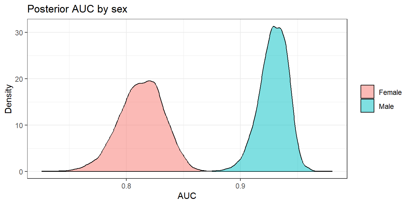
AUC by group
\(\text{AUC}_{A=0} = \text{AUC}_{A=1}\)
Equal discriminative ability
Why these metrics conflict
If the prevalence of the outcome differs between groups, it is mathematically impossible to achieve demographic parity, equalized odds, and predictive parity simultaneously. The appropriate metric depends on the application and ethical framework.
6.3 Computing fairness metrics from posterior draws
We continue with the Pima dataset and treat Sex (which we simulate here as it is not in the original dataset) as the protected attribute. In your own data, replace sex with the appropriate variable.
# The Pima dataset does not include sex; we simulate a binary sex variable# for illustration. In practice, use the actual subgroup variable in your data.set.seed(99)pima_test <- pima_test %>%mutate(sex =rbinom(n(), 1, 0.48)) # 0 = female, 1 = malecat("Subgroup sizes in test set:\n")
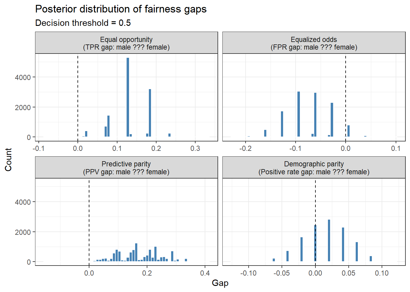
gap_vars <-c("TPR_diff", "FPR_diff", "PPV_diff", "PR_diff")gap_labels <-c("Equal opportunity\n(TPR gap: male ??? female)","Equalized odds\n(FPR gap: male ??? female)","Predictive parity\n(PPV gap: male ??? female)","Demographic parity\n(Positive rate gap: male ??? female)")gap_long <- fairness_df %>%select(all_of(gap_vars)) %>%pivot_longer(everything(), names_to ="metric", values_to ="gap") %>%mutate(metric =factor(metric, levels = gap_vars, labels = gap_labels))ggplot(gap_long, aes(x = gap)) +geom_histogram(bins =60, fill ="steelblue", colour ="white") +geom_vline(xintercept =0, linetype ="dashed", colour ="black") +facet_wrap(~ metric, scales ="free_x", ncol =2) +labs(title ="Posterior distribution of fairness gaps",subtitle =paste0("Decision threshold = ", tau),x ="Gap", y ="Count") +theme_bw()
The discrete/gapped pattern is expected. The fairness metrics (TPR, FPR, PPV, positive rate) are computed from counts within subgroups. With a fixed test set and fixed subgroup sizes, the possible values of these metrics are discrete fractions with a fixed denominator.
The Bayesian approach provides full posterior distributions over each fairness metric. Rather than a single point estimate of, say, the TPR gap, we can ask: “What is the probability that the true TPR gap exceeds 0.10?” This is directly answerable from the posterior and is far more informative for decision-making than a binary hypothesis test.
References
Bastos, Mayara Lisboa, Gamuchirai Tavaziva, Syed Kunal Abidi, Jonathon R Campbell, Louis-Patrick Haraoui, James C Johnston, Zhiyi Lan, et al. 2020. “Diagnostic Accuracy of Serological Tests for Covid-19: Systematic Review and Meta-Analysis.”Bmj 370.
Piironen, Juho, Markus Paasiniemi, Alejandro Catalina, Frank Weber, Osvaldo Martin, and Aki Vehtari. 2025. “projpred: Projection Predictive Feature Selection.”https://mc-stan.org/projpred/.