Code
dat <- read.table("data/Howell.txt", header = TRUE, sep = ";") %>%
mutate(male = factor(male, labels = c("female", "male")))brms, including prior specificationWhat is regression? (McElreath 2018)
Regression uses one or more predictor variables to model the distribution of an outcome variable.
In this lecture, we focus only on continuous outcomes, so we will use Bayesian linear regression.
The main ideas are the same as in ordinary linear regression:
What changes in the Bayesian framework is that:
For subject \(i\),
\[ Y_i \mid \mu_i, \sigma \sim N(\mu_i, \sigma) \]
with linear predictor
\[ \mu_i = \beta_0 + \beta_1 x_{i1} + \cdots + \beta_p x_{ip}. \]
Equivalently,
\[ Y_i = \mu_i + e_i, \qquad e_i \sim N(0, \sigma). \]
In practice, Bayesian workflow places strong emphasis on model checking, not only on writing down assumptions.
For a continuous outcome, a standard Bayesian linear regression model is
\[ Y_i \mid \mu_i, \sigma \sim N(\mu_i, \sigma) \]
\[ \mu_i = \beta_0 + \beta_1 x_{i1} + \cdots + \beta_p x_{ip}. \]
This model has two main components:
A two-group comparison is just a special case of linear regression.
If \(x_i = 0\) for group 1 and \(x_i = 1\) for group 2, then
\[ \mu_i = \beta_0 + \beta_1 x_i. \]
This is one reason why regression provides a unified framework for many familiar analyses.
We will use the Howell data on anthropometric measurements.
dat <- read.table("data/Howell.txt", header = TRUE, sep = ";") %>%
mutate(male = factor(male, labels = c("female", "male")))dat %>%
select(height, weight, age, male) %>%
tbl_summary(
statistic = list(
all_continuous() ~ "{mean} ({sd})",
all_categorical() ~ "{n} / {N} ({p}%)"
),
digits = all_continuous() ~ 2
)| Characteristic | N = 5441 |
|---|---|
| height | 138.26 (27.60) |
| weight | 35.61 (14.72) |
| age | 29.34 (20.75) |
| male | |
| female | 287 / 544 (53%) |
| male | 257 / 544 (47%) |
| 1 Mean (SD); n / N (%) | |
p1 <- ggplot(aes(x = weight, y = height), data = dat) +
  geom_point(size = 0.7, alpha = 0.7) +
  geom_smooth(se = FALSE)

p2 <- ggplot(aes(x = age, y = height), data = dat) +
  geom_point(size = 0.7, alpha = 0.7) +
  geom_smooth(se = FALSE)

p3 <- ggplot(aes(x = male, y = height), data = dat) +
  geom_boxplot()

ggarrange(p1, p2, p3, nrow = 1)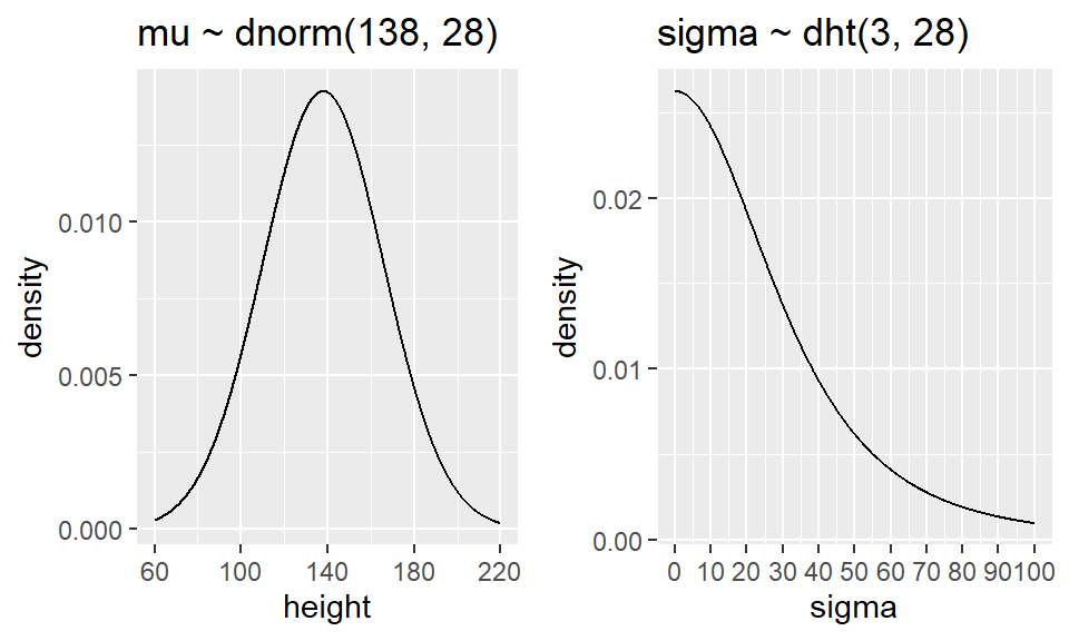
From these plots:
These plots suggest a model such as
\[ height_i \sim N(\mu_i, \sigma) \]
\[ \mu_i = \beta_0 + \beta_1\,weight_i + \beta_2\,age_i + \beta_3\,age_i^2 + \beta_4\,I(male_i = \text{male}). \]
For the Howell example, we will use the following weakly informative priors:
\[ \beta_0 \sim N(0, 100) \]
\[ \beta_j \sim N(0, 10), \qquad j=1,2,3,4 \]
\[ \sigma \sim \text{Student-}t(3, 0, 20), \qquad \sigma > 0 \]
These priors are broad enough to let the data dominate, but still give some regularization.
p1 <- tibble(x = seq(from = -350, to = 350, by = 0.2)) %>%
  ggplot(aes(x = x, y = dnorm(x, mean = 0, sd = 100))) +
  geom_line() +
  scale_x_continuous(breaks = seq(from = -300, to = 300, by = 100)) +
  labs(title = "Prior: N(0, 100)",
       y = "Density",
       x = "Intercept")

p2 <- tibble(x = seq(from = -35, to = 35, by = 0.1)) %>%
  ggplot(aes(x = x, y = dnorm(x, mean = 0, sd = 10))) +
  geom_line() +
  scale_x_continuous(breaks = seq(from = -35, to = 35, by = 5)) +
  labs(title = "Prior: N(0, 10)",
       y = "Density",
       x = expression(beta))

p3 <- tibble(x = seq(from = 0, to = 100, by = 0.1)) %>%
  ggplot(aes(x = x, y = 2 * dt(x / 20, df = 3) / 20)) +
  geom_line() +
  labs(title = "Prior: Student-t(3, 0, 20)",
       y = "Density",
       x = expression(sigma))

ggarrange(p1, p2, p3, nrow = 1)
brmsget_prior(
height ~ weight + age + I(age^2) + male,
data = dat,
family = gaussian()
) prior class coef group resp dpar nlpar lb ub tag
(flat) b
(flat) b age
(flat) b IageE2
(flat) b malemale
(flat) b weight
student_t(3, 148.6, 16) Intercept
student_t(3, 0, 16) sigma 0
source
default
(vectorized)
(vectorized)
(vectorized)
(vectorized)
default
defaultbrmsWe now fit the Bayesian linear regression model in brms.
fit1 <- brm(
  data = dat,
  family = gaussian(),
  height ~ weight + age + I(age^2) + male,
  prior = c(
    prior(normal(0, 100), class = "Intercept"),
    prior(normal(0, 10), class = "b"),
    prior(student_t(3, 0, 20), class = "sigma")
  ),
  iter = 10000,
  warmup = 5000,
  chains = 4,
  cores = 4,
  seed = 123,
  refresh = 0,
  silent = 2
)

saveRDS(fit1, "data/chp4_reg_example")brms formula meansThe formula
height ~ weight + age + I(age^2) + malemeans that:
I(age^2) adds a quadratic age termmale is treated as a factor, and brms creates the necessary indicator variable automaticallyfit1 <- readRDS("data/chp4_reg_example")
summary(fit1) Family: gaussian
Links: mu = identity
Formula: height ~ weight + age + I(age^2) + male
Data: dat (Number of observations: 544)
Draws: 4 chains, each with iter = 10000; warmup = 5000; thin = 1;
total post-warmup draws = 20000
Regression Coefficients:
Estimate Est.Error l-95% CI u-95% CI Rhat Bulk_ESS Tail_ESS
Intercept 75.52 1.00 73.54 77.48 1.00 22865 17295
weight 1.26 0.06 1.15 1.37 1.00 8032 11579
age 1.06 0.11 0.84 1.29 1.00 7384 10434
IageE2 -0.01 0.00 -0.01 -0.01 1.00 7736 11039
malemale 1.86 0.79 0.29 3.39 1.00 12359 12021
Further Distributional Parameters:
Estimate Est.Error l-95% CI u-95% CI Rhat Bulk_ESS Tail_ESS
sigma 8.70 0.27 8.19 9.24 1.00 14863 13046
Draws were sampled using sampling(NUTS). For each parameter, Bulk_ESS
and Tail_ESS are effective sample size measures, and Rhat is the potential
scale reduction factor on split chains (at convergence, Rhat = 1).Using posterior means, the fitted regression equation can be written approximately as
\[ \widehat{height}_i = \beta_0 + \beta_1\,weight_i + \beta_2\,age_i + \beta_3\,age_i^2 + \beta_4\,I(male_i = \text{male}). \]
Each coefficient is interpreted conditionally on the other predictors.
For example:
weight describes the expected change in height for a one-unit increase in weight, holding age and sex fixedmale describes the expected height difference between males and females of the same age and weightage and age^2 are includedWhat is the posterior evidence that males are taller than females, adjusting for age and weight?
hypothesis(fit1, "malemale > 0", alpha = 0.025)Hypothesis Tests for class b:
Hypothesis Estimate Est.Error CI.Lower CI.Upper Evid.Ratio Post.Prob Star
1 (malemale) > 0 1.86 0.79 0.29 3.39 104.82 0.99 *
---
'CI': 95%-CI for one-sided and 97.5%-CI for two-sided hypotheses.
'*': For one-sided hypotheses, the posterior probability exceeds 97.5%;
for two-sided hypotheses, the value tested against lies outside the 97.5%-CI.
Posterior probabilities of point hypotheses assume equal prior probabilities.What is the posterior evidence that males are taller than females by 2 cm, adjusting for age and weight?
hypothesis(fit1, "malemale > 2", alpha = 0.025)Hypothesis Tests for class b:
Hypothesis Estimate Est.Error CI.Lower CI.Upper Evid.Ratio Post.Prob
1 (malemale)-(2) > 0 -0.14 0.79 -1.71 1.39 0.74 0.43
Star
1
---
'CI': 95%-CI for one-sided and 97.5%-CI for two-sided hypotheses.
'*': For one-sided hypotheses, the posterior probability exceeds 97.5%;
for two-sided hypotheses, the value tested against lies outside the 97.5%-CI.
Posterior probabilities of point hypotheses assume equal prior probabilities.This is a nice example of a Bayesian probability statement that is more direct than a classical p-value.
plot(conditional_effects(fit1, "weight"), points = TRUE, point_args = list(size = 0.5))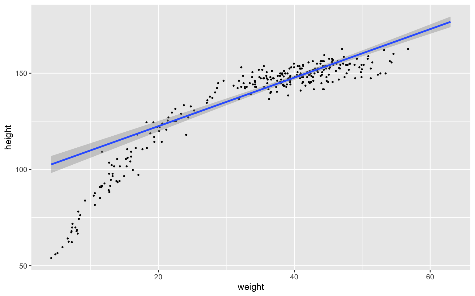
plot(conditional_effects(fit1, "age"), points = TRUE, point_args = list(size = 0.5))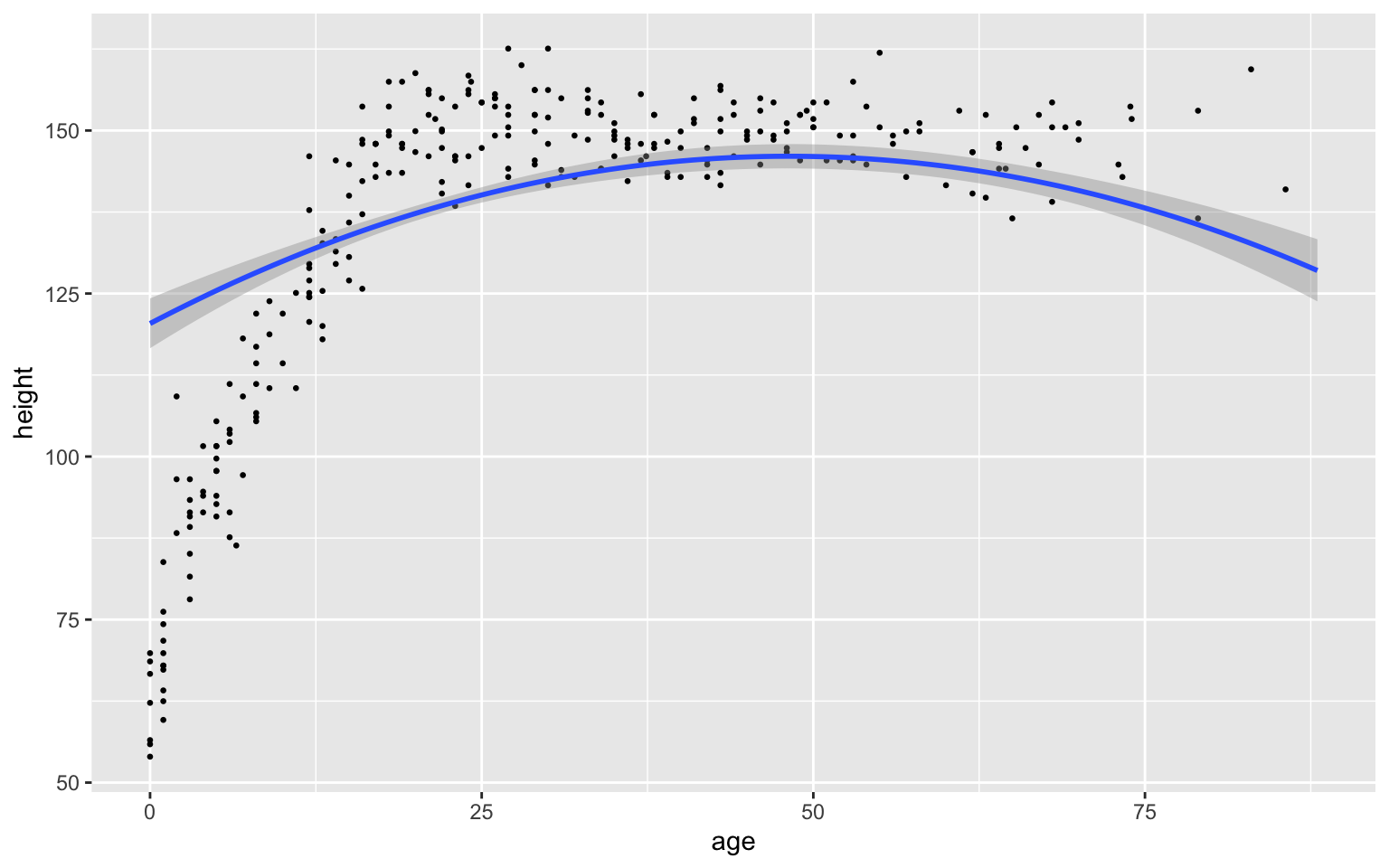
plot(conditional_effects(fit1, "male"))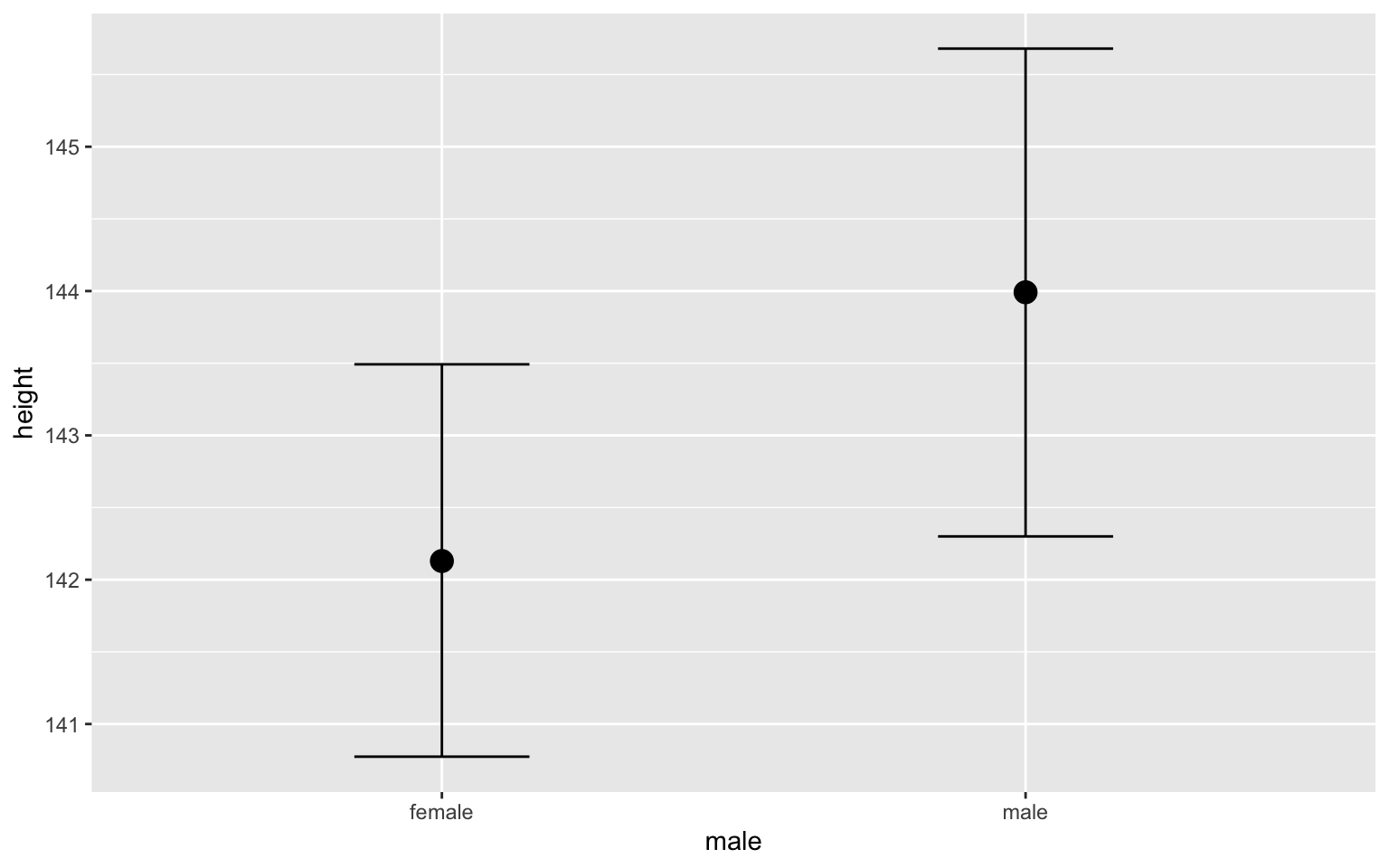
These plots are often easier to interpret than the coefficient table alone.
bayes_R2(fit1) Estimate Est.Error Q2.5 Q97.5
R2 0.9011375 0.002571426 0.8955066 0.9055716Bayesian \(R^2\) summarizes how much of the variation in the outcome is explained by the model, while accounting for posterior uncertainty.
Suppose we want to predict height for a female who is 33 years old and weighs 60 kg.
mean_pred <- posterior_epred(
  fit1,
  newdata = data.frame(weight = 50, age = 33, male = "female")
)

mean(mean_pred)
[1] 161.6473posterior_interval(mean_pred, prob = 0.95) 2.5% 97.5%
[1,] 160.2126 163.0788ind_predic <- posterior_predict(
fit1,
newdata = data.frame(weight = 50, age = 33, male = "female")
)
mean(ind_predic)[1] 161.6597posterior_interval(ind_predic, prob = 0.95) 2.5% 97.5%
[1,] 144.4122 178.8027mean(ind_predic > 160) #P(ind_predic > 160);[1] 0.57235posterior_epred() gives the posterior distribution of the mean outcomeposterior_predict() gives the posterior predictive distribution for a new observed outcomeThe predictive interval is wider because it includes both parameter uncertainty and residual variation.
Bayesian workflow puts strong emphasis on checking both:
plot(fit1)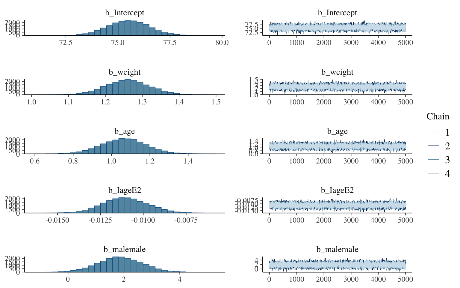
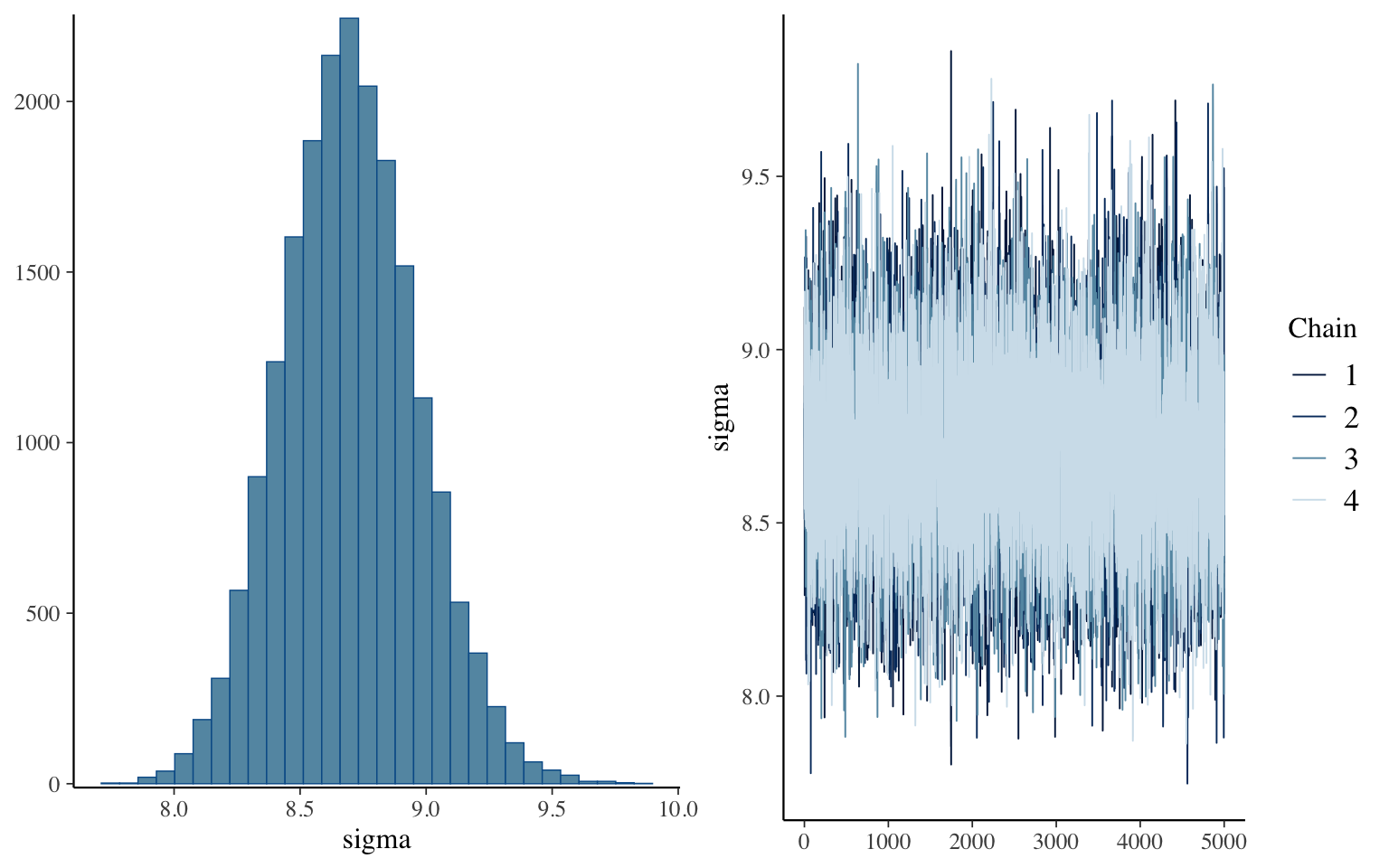
Useful diagnostics include:
summary(fit1)$fixed[, c("Rhat", "Bulk_ESS", "Tail_ESS")] Rhat Bulk_ESS Tail_ESS
Intercept 1.000293 22865.009 17294.68
weight 1.000921 8031.831 11579.04
age 1.001066 7384.440 10434.08
IageE2 1.000847 7735.917 11038.66
malemale 1.000326 12359.105 12020.54summary(fit1)$spec_pars[, c("Rhat", "Bulk_ESS", "Tail_ESS")] Rhat Bulk_ESS Tail_ESS
sigma 1.000058 14863.04 13046.32A good Bayesian model should generate replicated data that resemble the observed data.
pp_check(fit1, ndraws = 50)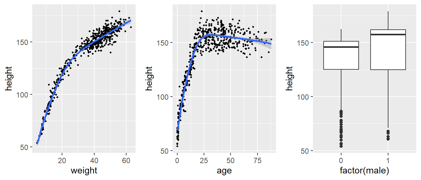
pp_check(fit1, type = "stat_2d", stat = c("max", "min"))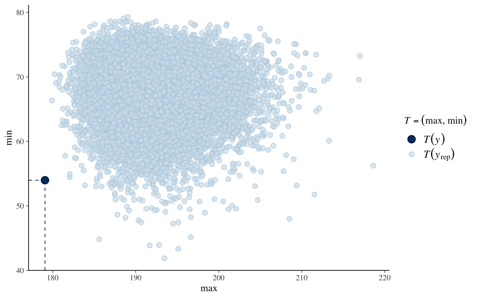
Questions to ask:
res_df <- fit1$data %>%
  mutate(
    predict_y = predict(fit1)[, "Estimate"],
    std_resid = residuals(fit1, type = "pearson")[, "Estimate"]
  )

ggplot(res_df, aes(predict_y, std_resid)) +
  labs(y = "Standardized residuals", x = "Fitted mean") +
  geom_point(size = 0.8) +
  stat_smooth(se = FALSE) +
  theme_bw()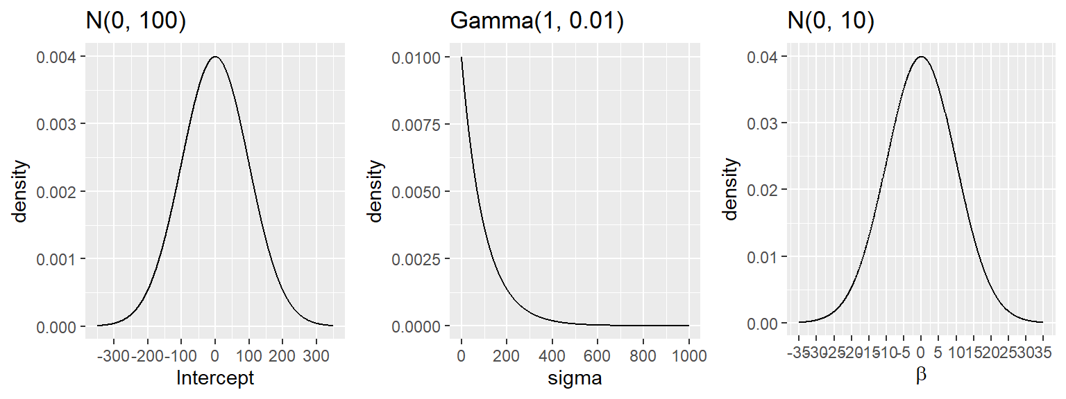
This plot helps assess:
pairs(
  fit1,
  off_diag_args = list(size = 0.5, alpha = 0.25)
)
If some coefficients are strongly correlated in the posterior, this may indicate:
We often compare multiple plausible regression models rather than assuming one model is automatically correct.
We compare two models:
fit2 <- brm(
  data = dat,
  family = gaussian(),
  height ~ weight + I(weight^2) + age + I(age^2) + male,
  prior = c(
    prior(normal(0, 100), class = "Intercept"),
    prior(normal(0, 10), class = "b"),
    prior(student_t(3, 0, 20), class = "sigma")
  ),
  iter = 10000,
  warmup = 5000,
  chains = 4,
  cores = 4,
  seed = 123,
  refresh = 0,
  silent = 2
)
saveRDS(fit2, "data/chp4_height2")Two common Bayesian model comparison tools are:
Both are based on predictive performance.
fit2 <- readRDS("data/chp4_height2")

waic1 <- waic(fit1)
waic2 <- waic(fit2)
compare_ic(waic1, waic2)
WAIC SE
fit1 3902.84 35.22
fit2 3383.70 38.88
fit1 - fit2 519.14 40.30loo1 <- loo(fit1)
loo2 <- loo(fit2)
loo_compare(loo1, loo2) elpd_diff se_diff
fit2 0.0 0.0
fit1 -259.6 20.1 Which model has better fit in this case?
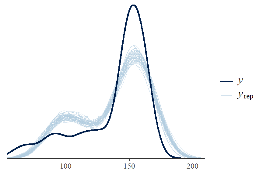
pp_check(fit2, ndraws = 50)Model comparison is not only about a numerical criterion. We should also ask whether the more flexible model improves fit in a meaningful way.
A quadratic term allows some curvature, but it imposes a specific shape.
A spline is more flexible. Instead of forcing a straight line or a quadratic curve, we allow the data to inform a smooth function.
In brms, this is specified using s(age).
brmsfit_spline <- brm(
data = dat,
family = gaussian(),
height ~ weight + s(age) + male,
prior = c(
prior(normal(0, 100), class = "Intercept"),
prior(normal(0, 10), class = "b"),
prior(student_t(3, 0, 20), class = "sigma")
),
iter = 10000,
warmup = 5000,
chains = 4,
cores = 4,
seed = 123,
refresh = 0,
silent = 2
)
saveRDS(fit_spline, "data/chp4_heightsp")fit_spline <- readRDS("data/chp4_heightsp")
plot(conditional_effects(fit_spline, "age"), points = TRUE, point_args = list(size = 0.5))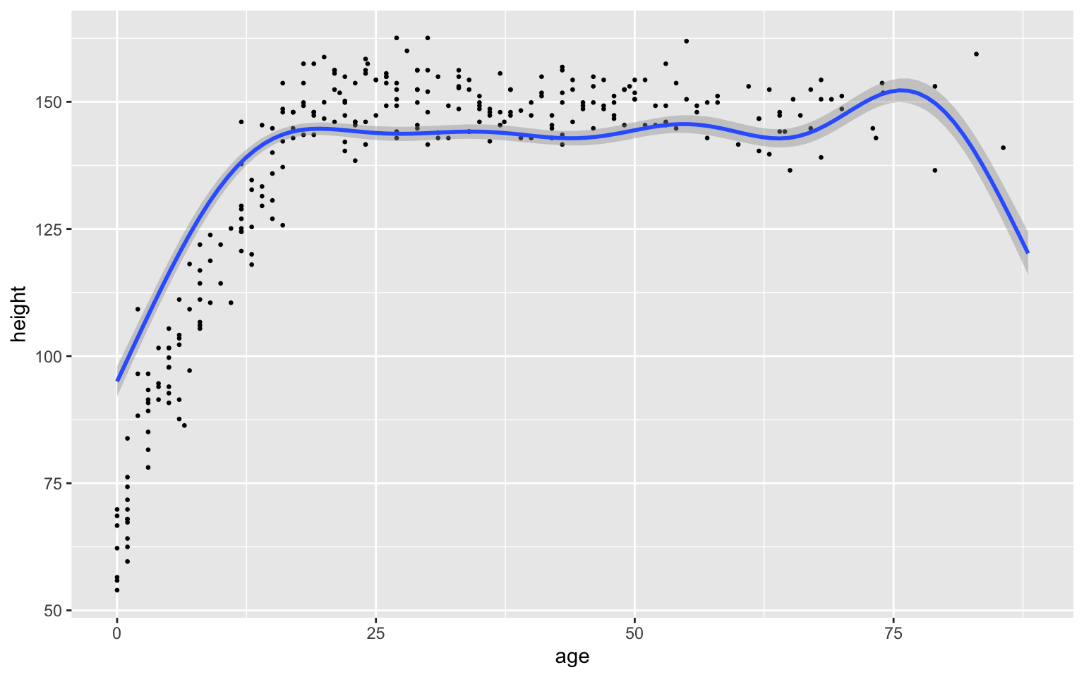
loo_spline <- loo(fit_spline)
loo_compare(loo2, loo_spline)
elpd_diff se_diff
fit_spline 0.0 0.0
fit2 -13.9 20.4 pp_check(fit_spline, ndraws = 50)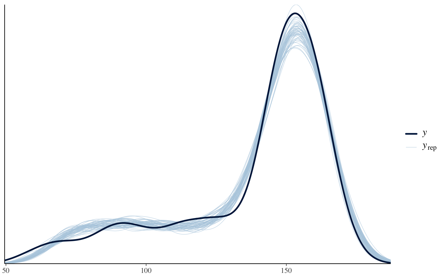
Splines are useful when:
Spline effects are usually interpreted graphically, not coefficient by coefficient.
When the number of predictors is large relative to the sample size, weak, standard priors can lead to:
Shrinkage priors pull many coefficients toward zero unless the data strongly support a larger effect.
The Bayesian lasso uses a Laplace prior on each regression coefficient:
\[ \beta_j \sim \text{Laplace}(0, \tau). \]
Compared with a normal prior, the Laplace prior places more mass near zero, so smaller coefficients are shrunk more strongly.
brms
In current brms workflow, shrinkage is commonly implemented using priors such as the horseshoe prior.
So in this lecture:
brms using the horseshoe prior, which is convenient and effective in practiceTo illustrate shrinkage, consider a linear regression with many candidate predictors, but only a few truly matter.
set.seed(123)

n <- 150
p <- 10

X <- matrix(rnorm(n * p), nrow = n, ncol = p)
colnames(X) <- paste0("x", 1:p)

sim_dat <- as_tibble(X) %>%
mutate(y = 2 * x1 - 1.5 * x3 + 1.2 * x7 + rnorm(n, sd = 2))fit_full <- brm(
y ~ .,
data = sim_dat,
family = gaussian(),
prior = c(
prior(normal(0, 5), class = "Intercept"),
prior(normal(0, 2), class = "b"),
prior(student_t(3, 0, 5), class = "sigma")
),
iter = 5000,
warmup = 2500,
chains = 4,
cores = 4,
seed = 123,
refresh = 0
)
fit_hs <- brm(
y ~ .,
data = sim_dat,
family = gaussian(),
prior = c(
prior(normal(0, 5), class = "Intercept"),
prior(horseshoe(par_ratio = 3 / 10), class = "b"),
prior(student_t(3, 0, 5), class = "sigma")
),
iter = 5000,
warmup = 2500,
chains = 4,
cores = 4,
seed = 123,
refresh = 0
)
saveRDS(fit_full, "data/chp4_vs_full")
saveRDS(fit_hs, "data/chp4_vs_hs")fit_full <- readRDS("data/chp4_vs_full")
fit_hs <- readRDS("data/chp4_vs_hs")
coef_full <- as.data.frame(fixef(fit_full)) %>%
rownames_to_column("term") %>%
filter(term != "Intercept") %>%
transmute(term, estimate = Estimate, lower = Q2.5, upper = Q97.5, model = "regular prior")
coef_hs <- as.data.frame(fixef(fit_hs)) %>%
rownames_to_column("term") %>%
filter(term != "Intercept") %>%
transmute(term, estimate = Estimate, lower = Q2.5, upper = Q97.5, model = "Horseshoe prior")
coef_plot <- bind_rows(coef_full, coef_hs) %>%
mutate(term = fct_reorder(term, estimate))
ggplot(coef_plot, aes(x = estimate, y = term, xmin = lower, xmax = upper, colour = model)) +
geom_point(position = position_dodge(width = 0.5)) +
geom_errorbarh(position = position_dodge(width = 0.5), height = 0) +
geom_vline(xintercept = 0, linetype = "dashed", colour = "grey50") +
labs(x = "Posterior estimate", y = NULL, colour = NULL)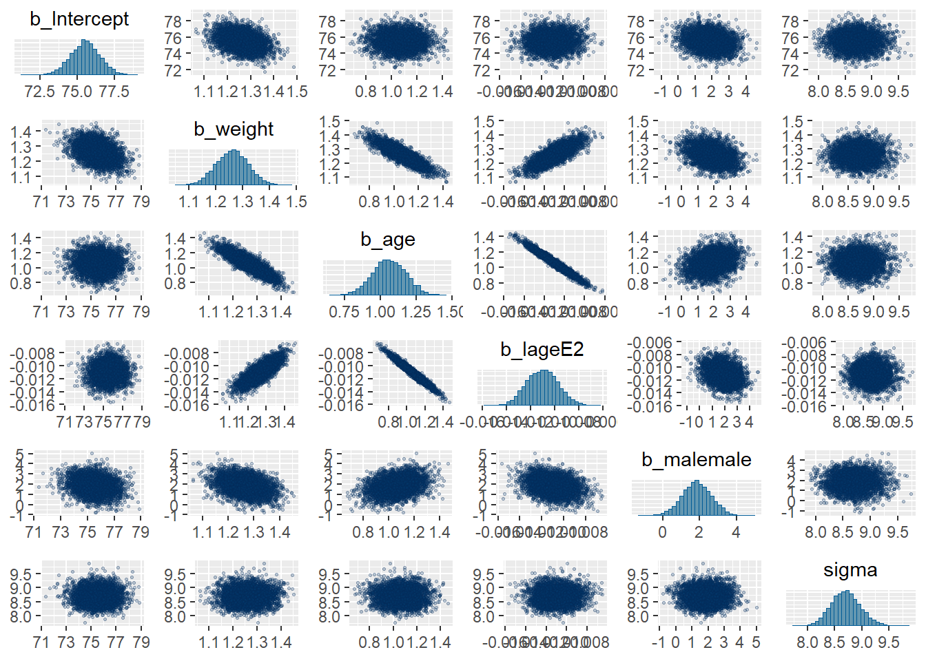
loo_full <- loo(fit_full)
loo_hs   <- loo(fit_hs)
loo_compare(loo_full, loo_hs)
elpd_diff se_diff
fit_hs 0.0 0.0
fit_full -1.7 1.7 The shrinkage model may improve out-of-sample prediction by shrinking noise coefficients more aggressively toward zero.
projpred package implements this ??? it projects the full posterior onto submodels and finds the minimal set of variables that preserves predictive performance without refitting in the model. (Package website)[https://mc-stan.org/projpred/index.html] (Piironen et al. 2025)h <- c("x1 > 0","x2 > 0","x3 > 0","x4 > 0","x5 > 0","x6 > 0","x7 > 0","x8 > 0","x9 > 0","x10 > 0")
hypothesis(fit_hs, h) # P(effect exceeds MCID)Hypothesis Tests for class b:
Hypothesis Estimate Est.Error CI.Lower CI.Upper Evid.Ratio Post.Prob Star
1 (x1) > 0 1.81 0.17 1.52 2.10 Inf 1.00 *
2 (x2) > 0 -0.09 0.14 -0.36 0.08 0.36 0.27
3 (x3) > 0 -1.30 0.16 -1.58 -1.03 0.00 0.00
4 (x4) > 0 -0.05 0.12 -0.27 0.12 0.55 0.35
5 (x5) > 0 -0.02 0.10 -0.21 0.14 0.73 0.42
6 (x6) > 0 -0.05 0.11 -0.27 0.10 0.49 0.33
7 (x7) > 0 1.45 0.16 1.20 1.72 Inf 1.00 *
8 (x8) > 0 0.12 0.14 -0.05 0.40 4.29 0.81
9 (x9) > 0 -0.15 0.15 -0.44 0.04 0.19 0.16
10 (x10) > 0 -0.03 0.11 -0.23 0.14 0.72 0.42
---
'CI': 90%-CI for one-sided and 95%-CI for two-sided hypotheses.
'*': For one-sided hypotheses, the posterior probability exceeds 95%;
for two-sided hypotheses, the value tested against lies outside the 95%-CI.
Posterior probabilities of point hypotheses assume equal prior probabilities.library(projpred)
ncores = 10
refm_obj <- get_refmodel(fit_hs)
# via cross-validation;
cv_fits <- run_cvfun(refm_obj, k=4)
# For running projpred's CV in parallel (see cv_varsel()'s argument `parallel`):
# Note: Parallel processing is disabled during package building to avoid issues
use_parallel <- FALSE # Set to TRUE for actual parallel processing
if (use_parallel) {
doParallel::registerDoParallel(ncores)
}
# Final cv_varsel() run:
cvvs <- cv_varsel(
refm_obj,
cv_method = "kfold",
cvfits = cv_fits,
### for the sake of speed (not recommended in general):
method = "L1",
nclusters_pred = 10,
###
nterms_max = 8,
parallel = use_parallel,
### In interactive use, we recommend not to deactivate the verbose mode:
verbose = 0
###
)
# Tear down the CV parallelization setup:
if (use_parallel) {
doParallel::stopImplicitCluster()
foreach::registerDoSEQ()
}
options(projpred.plot_vsel_show_cv_proportions = TRUE)
plot(cvvs, stats = "mlpd", deltas = TRUE)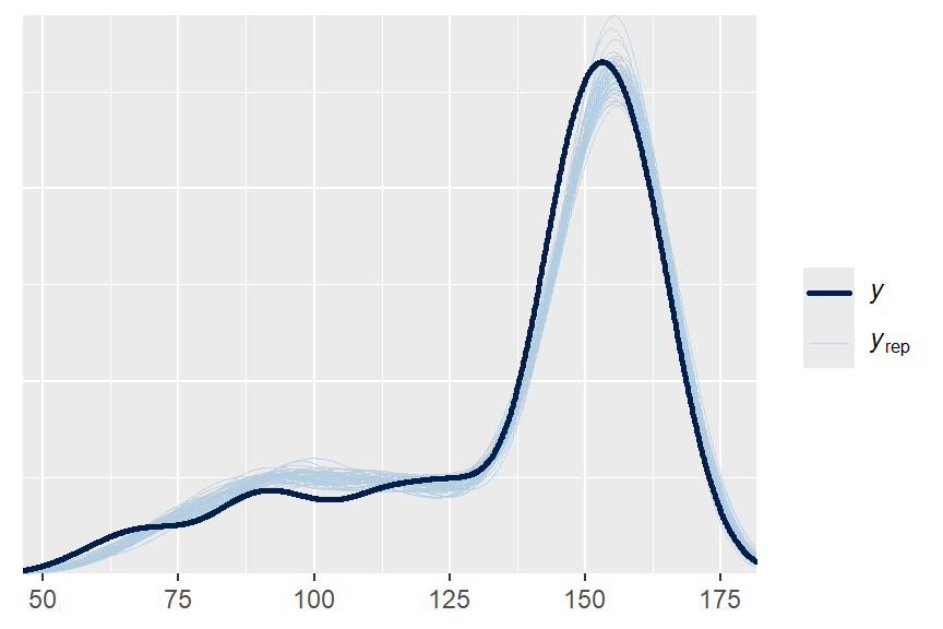
suggest_size(cvvs, stat = "mlpd") # suggested minimal variable set;[1] 3ranking(cvvs) #ranking of the top predictors across validation set;$fulldata
[1] "x1" "x3" "x7" "x9" "x8" "x2" "x6" "x4"
$foldwise
[,1] [,2] [,3] [,4] [,5] [,6] [,7] [,8]
[1,] "x1" "x3" "x7" "x9" "x8" "x2" "x4" "x6"
[2,] "x1" "x7" "x3" "x2" "x9" "x5" "x4" "x8"
[3,] "x1" "x7" "x3" "x4" "x8" "x2" "x9" "x5"
[4,] "x1" "x3" "x7" "x9" "x8" "x2" "x5" "x4"
[5,] "x1" "x7" "x3" "x6" "x9" "x8" "x2" "x4"
attr(,"class")
[1] "ranking"