Lecture 1 - Introduction to Bayesian anaysis

Learning Objectives
  • Students and instructor introduction
  • Going over course syllabus
  • Introduce Bayesian inference from a clinical researcher’s perspective.
  • Reviewing Probability and Other statistical concepts

About me

My primary research focuses on developing methodology for statistical inference with complex longitudinal data in comparative effectiveness research. My areas of methodological interest include causal inference, Bayesian statistics, longitudinal data analysis, and mixture and joint modelling.

Introducing Yourself

You can share your program, learning goals, and hobby.

Detailed course syllabus is posted on Quercus.

1. Introduction to Bayesian Reasoning

1.1 Refreshing Frequentist Inference

Most of us were trained in the frequentist tradition. Before we introduce a new way of thinking, let us revisit what we already know.

A Clinical Example: Phase I Dose Escalation

Working Example - Frequentist Approach

Suppose you have observed 20 patients in a Phase I RCT on a given dose of drug,

  • 0 out of 20 patients have had an adverse event (\(= 0\%\))
  • Decision to escalate to a higher dose if it is unlikely that the current dosing results in a true proportion of adverse events above 20%
  • This is a classic phase I estimate. Let \(\theta\) be the true risk of adverse event (parameter of interest).
  • Under the frequentist framework (One-sided Exact Binomial Test), we test \(H_0: \theta = 0.2\) vs \(H_a: \theta \leq 0.2\).
  • If \(H_0\) is true, we would expect to see \(0.2 \times 20 = 4\) patients experiencing AE. The p-value considers the probability of seeing an outcome as extreme or more extreme than the observed 0 AE.

\[P\text{-value} = P(Y=0) = {20 \choose 0} 0.2^0 \times 0.8^{20} = 0.0115\]

  • With a significance level of \(5\%\), we reject \(H_0\) and decide to escalate the dose.
Code
binom.test(x = 0, n = 20, p = 0.2, alternative = "less")

    Exact binomial test

data:  0 and 20
number of successes = 0, number of trials = 20, p-value = 0.01153
alternative hypothesis: true probability of success is less than 0.2
95 percent confidence interval:
 0.0000000 0.1391083
sample estimates:
probability of success 
                     0 
Code
# P-value using binomial probability
pbinom(q = 0, size = 20, p = 0.2, lower.tail = TRUE)
[1] 0.01152922
  • The observed proportion \(\hat{\theta} = 0\) with 95% CI: 0 – 0.14.

What does this output actually mean?

Quiz: Interpreting the P-value

Given the p-value = 0.012 from the binomial exact test, which of the following are true?

  1. The probability that the null hypothesis is true is 1.2%.
  2. The probability that the alternative hypothesis is true is 1 - 1.2% = 98.8%.
  3. There is a 1.2% chance of making a mistake by rejecting the null hypothesis.
  4. Assuming the risk of AE is 0.2 (\(H_0\) is true), we would obtain a sample estimated risk of AE as extreme or more than the observed 0%, in 1.2% of studies in the long run when repeating the trial.
Quiz: Interpreting the Confidence Interval

Given the 95% CI of \(\theta\) is (0, 0.14), which of the following are true?

  1. If we recruit another sample of 20 patients, there is a 95% chance the sample proportion of AE would be between 0% and 14%.
  2. About 95% of patients in the sample will have a risk of AE between 0 and 14%.
  3. We are 95% confident that the interval (0, 0.14) captured the true risk of AE.
  4. If we repeat this trial many times, then about 95% of the intervals produced will capture the true risk of AE.

1.2 Questions We Want to Answer But Cannot

The frequentist framework is powerful and well-established. But after seeing that output, does it answer the questions a clinician or clinical researcher actually has?

Consider what we really want to know in the Phase I example:

  1. What is the probability that the true AE rate is below 20%, given what we just observed?
  2. What is the probability this drug is safe enough to escalate?
  3. If I had some prior knowledge about this drug class, how should that change my conclusion?
  4. A patient asks: “What are the chances this treatment is safe for me?” and what does your analysis let you say?

The honest frequentist answer to all four questions is: I cannot tell you. Not because the methods are wrong, but because they were never designed to answer these questions.

What frequentist methods can and cannot say
Frequentist What we actually want
Parameter \(\theta\) Fixed unknown constant A quantity we can assign probability to
Prior knowledge Informal; Hypothesis driven Formally incorporated
Direct probability statement about \(\theta\)? ❌ Not possible, what we get: \(P(\text{data this extreme} \mid H_0 \text{ true})\) ✅ This is what we want, e.g., \(P( parameter > MCID \mid \text{data})\)
95% CI 95% of future intervals contain \(\theta\) 95% probability \(\theta\) is in this interval
  • The p-value tells us how surprised we should be by the data if the null were true. It does not tell us how likely the null is to be true.

  • As Wasserstein and Lazar (2016) note, “p-values do not measure the probability that the studied hypothesis is true.”


1.3 Bayesian Reasoning - A Different Way of Thinking

The Bayesian framework is built around a simple and intuitive idea:

We start with a belief. We observe data. We update our belief.

To summarize conceptually
  • The Bayesian approach provides an updated belief as a weighted combination of prior beliefs regarding that state and the currently available evidence, with the possibility of the current evidence overwhelming prior beliefs, or prior beliefs remaining largely intact in the face of scant evidence.

\[\text{updated belief} = \text{current evidence} \times \text{prior belief or evidence}\]

This is not a new idea, it is how humans naturally reason under uncertainty.

  • A doctor revises their diagnosis as new test results come in.
  • A regulator updates their confidence in a drug as trial data accumulate.

Bayesian statistics formalizes this process using probability.

High-level Bayesian reasoning for the AE example

Returning to our Phase I example:

  • Before seeing data: we have some belief about \(\theta\), the true AE rate. Perhaps we think all values between 0 and 1 are equally plausible (a flat, uninformative prior). Or perhaps we have some prior clinical experience suggesting the rate is likely low.

  • We observe data: 0 out of 20 patients experienced an AE.

  • We update our belief: combining what we knew before with what we just observed, we obtain a posterior distribution for \(\theta\). This is a full probability distribution over all possible values of \(\theta\), not just a point estimate.

  • We answer the clinical question directly: from the posterior, we can compute \(P(\theta < 0.20 \mid \text{data})\) directly. This is the probability that the true AE rate is below 20%, given everything we know.

What the Bayesian framework gives us

More about Beta-binomial model next week. For illustration, from the posterior distribution \(Beta(1, 21)\), we can directly compute:

Code
# Posterior: Beta(1, 21) given prior Beta(1,1) and x=0, n=20
a_post <- 1 + 0
b_post <- 1 + 20

# Posterior mean
cat("Posterior mean:", round(a_post / (a_post + b_post), 3), "\n")
Posterior mean: 0.045 
Code
# 95% Credible Interval
cat("95% Credible Interval:",
    round(qbeta(c(0.025, 0.975), a_post, b_post), 3), "\n")
95% Credible Interval: 0.001 0.161 
Code
# Direct answer to the clinical question
cat("P(theta < 0.20 | data):",
    round(pbeta(0.20, a_post, b_post), 3), "\n")
P(theta < 0.20 | data): 0.991 

\(P(\theta < 0.20 \mid \text{data}) = 0.99\) means there is a 99% posterior probability that the true AE rate is below 20%. We can now directly and confidently recommend dose escalation.

This is the kind of direct probability statement that clinical researchers and regulators find intuitive and actionable.


1.4 The Growing Role of Bayesian Analysis in Clinical Research

Bayesian methods are not new, they date back to the Reverend Thomas Bayes in the 18th century. But their adoption in clinical research has accelerated dramatically in recent decades, driven by three forces:

1. Computational advances. Modern Markov Chain Monte Carlo (MCMC) methods and software (Stan, JAGS, brms in R) have made Bayesian analysis of complex models practical for applied researchers.

2. Regulatory acceptance. The FDA Center for Devices and Radiological Health finalized Bayesian guidance for medical device trials in 2010. Bayesian adaptive designs have been increasingly used in oncology, rare disease, and pediatric trials where small sample sizes make frequentist inference particularly limited (Lee et al. 2026).

3. Recognition of frequentist limitations. The American Statistical Association’s 2016 statement on p-values (Wasserstein and Lazar 2016) and its 2019 follow-up (Wasserstein, Schirm, and Lazar 2019) sparked widespread reflection on over-reliance on p-values and arbitrary significance thresholds, opening the door for Bayesian alternatives.

Bayesian methods in clinical trials
  • Adaptive designs: Bayesian posterior probabilities guide interim decisions on sample size, dose allocation, and early stopping.
  • Borrowing historical information: Bayesian hierarchical models formally incorporate evidence from prior studies, reducing required sample sizes in rare disease trials.
  • Pediatric and rare disease research: where randomizing large samples is ethically or practically impossible, Bayesian methods allow principled use of adult data or natural history data to inform inference.
  • Biomarker and platform trials: Bayesian methods power modern basket and umbrella trial designs that evaluate multiple treatments or subgroups simultaneously.

By the end of this course, you will have the tools to read, critically evaluate, and conduct Bayesian analyses in your own clinical research.

2. Probability, random variables and distributions

2.1. Thinking like a Bayesian using the concept of probability

Probability is not unitary

  • Mathematically probability is clearly defined (a quantity between 0 and 1)
  • There are a few ways of interpreting probability, most notably, long run relative frequency and subjective probability.
Probability

1. Long run relative frequency

The classical or frequentist way of interpreting probability is based on the proportion of times an outcome occurs in a large (i.e. approaching infinity) number of repetitions of an experiment.

  • This view has various serious problems, including that it requires the outcome to be observable and the “experiment” to be indeed repeatable!

2. Subjective probability

The alternative way (essentially proposed by Bayes, LaPlace, other later prominent Bayesians) is the subjective probability.

  • It encompasses one’s views, opinions or beliefs about an event or statement.
  • This event does not have to be repeatable or the outcome observable.
  • It is based on belief.
  • Using this approach, we can express the uncertainty around parameters using probability distributions (e.g., beta distribution for the risk \(\theta\) of death after an operation)

2.2 Probability

Probability has a central place in Bayesian analysis

  • we put a prior probability distribution on the unknowns (parameters),
  • we model the observed data with a probability distribution (likelihood),
  • and we combine the two into a posterior probability distribution
Probability Terminology

(Evans and Rosenthal 2004)

  • Sample space This set of all possible outcomes of an experiment/trial is known as the sample space of the experiment/trial and is denoted by \(S\) or \(\Omega\).

  • Experiment/Trial: each occasion we observe a random phenomenon that we know what outcomes can occur, but we do not know which outcome will occur

  • Event: Any subset of the sample space \(S\) is known as an event, denoted by \(A\). Note that, \(A\) is also a collection of one or more outcomes.

  • Probability defined on events: For each event \(A\) of the sample space \(S\), \(P(A)\), the probability of the event \(A\), satisfies the following three conditions:

    1. \(0 \leq P(A) \leq 1\)
    2. \(P(S) = 1\) and \(P(\emptyset) = 0\); \(\emptyset\) denotes the empty set
    3. \(P\) is (countably) additive, meaning that if \(A_1, A_2, \ldots\) is a finite or countable sequence of disjoint (also known as mutually exclusive events), then \[P(A_1 \cup A_2 \cup \ldots ) = P(A_1)+P(A_2)+\ldots\]
  • Union: Denote the event that either \(A\) or \(B\) occurs as \(A\cup B\).

  • Intersection: Denote the event that both \(A\) and \(B\) occur as \(A\cap B\)

  • Complement: Denote the event that \(A\) does not occur as \(\bar{A}\) or \(A^{C}\) or \(A^\prime\) (different people use different notations)

  • Disjoint (or mutually exclusive): Two events \(A\) and \(B\) are said to be disjoint if the occurrence of one event precludes the occurrence of the other. If two events are mutually exclusive, then \(P(A\cup B)=P(A)+P(B)\)

Example

Sample Space

  1. If the experiment consists of the flipping of a coin, then \[ S = \{H, T\}\]
  2. If the experiment consists of rolling a die, then the sample space is \[ S = \{1, 2, 3, 4, 5, 6\}\]
  3. If the experiments consists of flipping two coins, then the sample space consists of the following four points: \[ S = \{(H,H), (H,T), (T,H), (T,T)\}\]

Event

  1. In Example (1), if E = {H}, then E is the event that a head appears on the flip of the coin. Similarly, if \(E = \{T \}\), then \(E\) would be the event that a tail appears
  2. In Example (2), if \(E = \{1\}\), then \(E\) is the event that one appears on the roll of the die. If \(E = \{2, 4, 6\}\), then \(E\) would be the event that an even number appears on the roll.
  3. In Example (3), if \(E = \{(H, H), (H, T )\}\), then \(E\) is the event that a head appears on the first coin.

Probability of an event. Let \(R\) be the sum of two standard dice. Suppose we are interested in \(P(R \le 4)\). Notice that the pair of dice can fall 36 different ways (6 ways for the first die and six for the second results in 6x6 possible outcomes, and each way has equal probability \(1/36\). \[\begin{aligned} P(R \le 4 ) &= P(R=2)+P(R=3)+P(R=4) \\ &= P(\left\{ 1,1\right\} )+P(\left\{ 1,2\right\} \mathrm{\textrm{ or }}\left\{ 2,1\right\} )+P(\{1,3\}\textrm{ or }\{2,2\}\textrm{ or }\{3,1\}) \\ &= \frac{1}{36}+\frac{2}{36}+\frac{3}{36} \\ &= \frac{6}{36} \\ &= \frac{1}{6} \end{aligned}\]

Probability Rules

General Addition Rule: \(P(A\cup B)=P(A)+P(B)-P(A\cap B)\)

The reason behind this fact is that if there is if \(A\) and \(B\) are not disjoint, then some area is added twice when we calculate \(P\left(A\right)+P\left(B\right)\). To account for this, we simply subtract off the area that was double counted. If \(A\) and \(B\) are disjoint, \(P(A\cup B)=P(A)+P(B)\).

Complement Rule: \(P(A)+P(A^c)=1\)

This rule follows from the partitioning of the set of all events (\(S\)) into two disjoint sets, \(A\) and \(A^c\). We learned above that \(A \cup A^c = S\) and that \(P(S) = 1\). Combining those statements, we obtain the complement rule.

Completeness Rule: \(P(A)=P(A\cap B)+P(A\cap B^c)\)

This identity is just breaking the event \(A\) into two disjoint pieces.

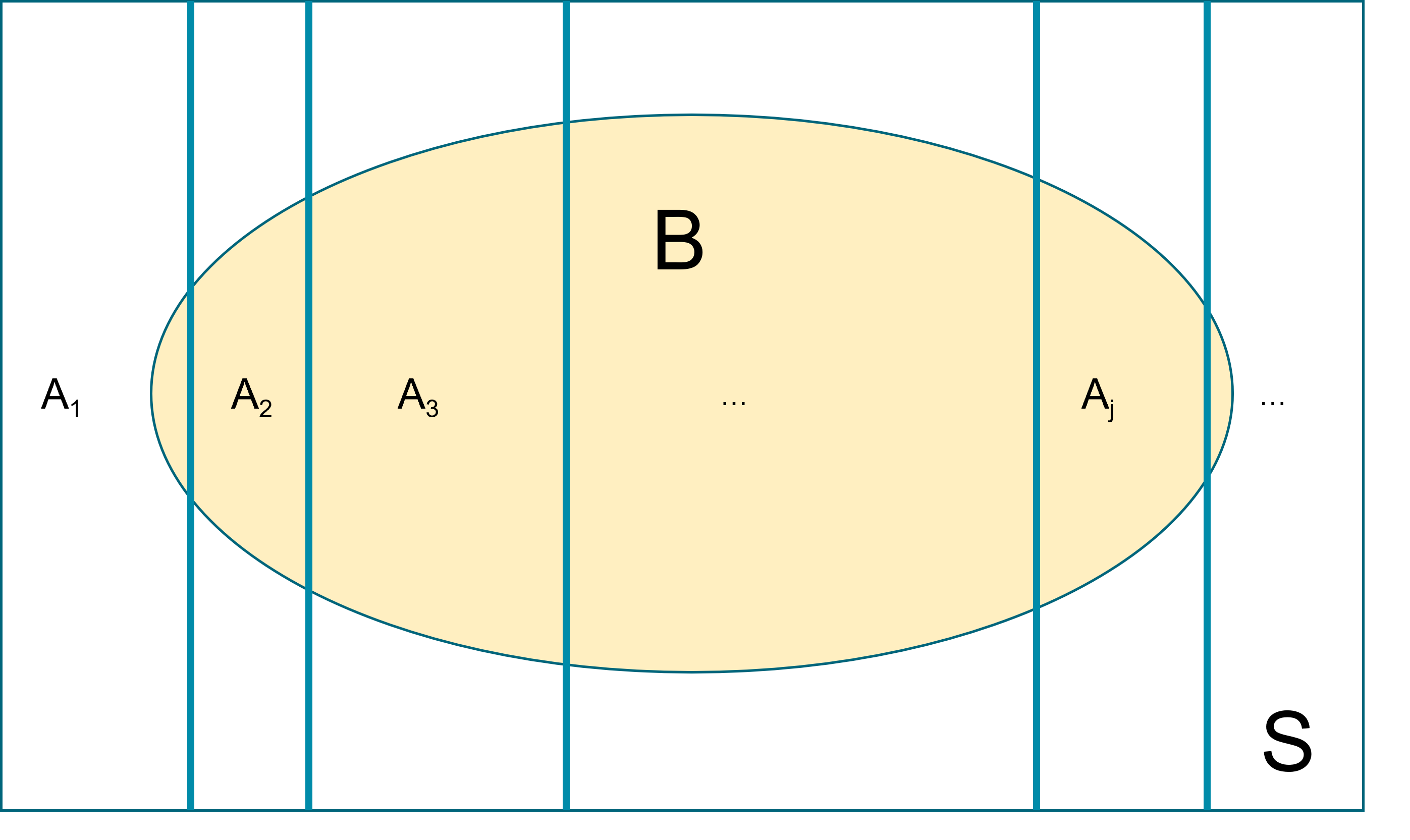
Law of total probability (unconditioned version): Let \(A_1, A_2, \ldots\) be events that form a partition of the sample space \(S\), Let \(B\) be any event. Then, \[P(B) = P(A_1 \cap B) + P(A_2 \cap B) + \ldots. \]

This law is key in deriving the marginal event probability in Bayes’ rule. Recall the HIV example from session 1, we have \(P(T^+) = P(T^+ \cap D^+)+P(T^+ \cap D^-)\).

Figure 1: Demonstrate Law of total probabiliy using Venn Diagram

Conditional Probability: The probability of even \(A\) occurring under the restriction that \(B\) is true is called the conditional probability of \(A\) given \(B\). Denoted as \(P(A|B)\).

In general we define conditional probability (assuming \(P(B) \ne 0\)) as \[P(A|B)=\frac{P(A\cap B)}{P(B)}\] which can also be rearranged to show \[\begin{aligned} P(A\cap B) &= P(A\,|\,B)\,P(B) \\ &= P(B\,|\,A)\,P(A) \end{aligned}\]

  • Because the order doesn’t matter and \(P\left(A\cap B\right)=P\left(B\cap A\right)\).
  • \(P(A|B) = 1\) means that the event \(B\) implies the event \(A\).
  • \(P(A|B) = 0\) means that the event \(B\) excludes the possibility of event \(A\).
Law of Total Probability

Suppose I know that whenever it rains there is 10% chance of being late at work, while the chance is only 1% if it does not rain. Suppose that there is 30% chance of raining tomorrow; what is the chance of being late at work?

Denote with event \(A\) as “I will be late to work tomorrow” and event \(B\) as “It is going to rain tomorrow”

\[\begin{aligned} P(A) &= P(A\mid B)P(B) + P(A \mid B^c) P(B^c) \\ &= 0.1\times 0.3+0.01\times 0.7=0.037 \end{aligned}\]

Independent: Two events \(A\) and \(B\) are said to be independent if \(P(A\cap B)=P(A)P(B)\).

What independence is saying that knowing the outcome of event \(A\) doesn’t give you any information about the outcome of event \(B\). If \(A\) and \(B\) are independent events, then \(P(A|B) = P(A)\) and \(P(B|A) = P(B)\).

In simple random sampling, we assume that any two samples are independent. In cluster sampling, we assume that samples within a cluster are not independent, but clusters are independent of each other.

  • Assumptions of independence and non-independence in statistical modelling are important.

  • In linear regression, for example, correct standard error estimates rely on independence amongst observations.

  • In analysis of clustered data, non-independence means that standard regression techniques are problematic.

Bayes’ Rule: This arises naturally from the rule on conditional probability. Since the order does not matter in \(A \cap B\), we can rewrite the equation:

\[\begin{aligned} P(A\mid B) &= \frac{P(A \cap B) }{P(B)}\\ &= \frac{P(B \cap A)}{P(B)}\\ &= \frac{P(B\mid A)P(A) }{P(B)}\\ &= \frac{P(B\mid A)P(A) }{P(B \cap A) + P(B \cap A^C)}\\ &= \frac{P(B\mid A)P(A) }{P(B\mid A)P(A) + P(B\mid A^C)P(A^C)} \end{aligned}\]

How to define and assign probabilities in general?

  1. Frequency-type (Empirical Probability): based on the idea of frequency or long-run frequency of an event.

    • Observe sequence of coin tosses (trials) and the count number of times of event \(A=\{H\}\). The relative frequency of \(A\) is given as, \[ P(A) = \frac{\text{Number of times A occurs}}{\text{Total number of trials}}. \]
    • Trials are independent. Relative frequency is unpredictable in short-term, but in long-run it’s predicable. Let \(n\) be the total number of trials and \(m\) be number of heads, then we have \[ P(A) = \lim_{n \rightarrow \infty} \frac{m}{n}.\]
    • Theoretical Probability: Sometimes \(P(A)\) can be deduced from mathematical model using uniform probability property on finite spaces.
      • If the sample space S is finite, then one possible probability measure on \(S\) is the uniform probability measure, which assigns probability \(1/|S|\), equal probability to each outcome. Here |S| is the number of elements in the sample space \(S\). By additivity, it then follows that for any event \(A\) we have,

    \[ P(A) = \frac{|A|}{|S|} = \frac{\text{Number of outcomes in S that satisfy A}}{\text{Total number of outcomes in S} } \]

    • Long-term frequency It is natural to think of large sequences of similar events defining frequency-type probability if we allow the number of trials to be indefinitely large.
Code
n = 1000
pHeads =0.5
set.seed(123)
flipSequence = sample( x=c(0,1),prob = c(1-pHeads,pHeads),size=n,replace=T)
 
r = cumsum(flipSequence)
n= 1:n
runProp = r/n
 
flip_data <- data.frame(run=1:1000,prop=runProp)

ggplot(flip_data,aes(x=run,y=prop,frame=run)) + 
  geom_path()+
  xlim(1,1000)+ylim(0.0,1.0)+
  geom_hline(yintercept = 0.5)+
  ylab("Proportion of Heads")+
  xlab("Number of Flips")+
  theme_bw()
Figure 2: Demonstrate law of large number with the coin tossing example
  1. Belief-type (Subjective Probability): based on the idea of degree of belief (weight of evidence) about an event where the scale is anchored at certain (=1) and impossible (=0).

  2. Which probability to use?

  • For inference, the Bayesian approach relies mainly on the belief interpretation of probability.

  • The laws of probability can be derived from some basic axioms that do not rely on long-run frequencies.

2.3 Probability Distributions

Random variables are used to describe events and their probability. The formal definition just means that a random variable describes how numbers are attached to each possible elementary outcome. Random variables can be divided into two types:

  • Continuous Random Variables: the variable takes on numerical values and could, in principle, take any of an uncountable number of values. These typically have values that cannot be counted, e.g. age, height, blood pressure, etc.

  • Discrete Random Variables: the variable takes on one of small set of values (or only a countable number of outcomes).

The value of a particular measurement can be thought of as being determined by chance, even though there may be no true randomness

  • a patient’s survival time after surgery for prostate cancer
  • distance an elderly person walks in 6 minutes
    • known factors may give an expected value and variance
    • unknown (or unknowable factors) lead to uncertainty given this mean
  • the component that appears random to the analyst is modelled as being random.

Probability distributions

  • The true distribution of most random variables (outcomes) is not known.
  • It is convenient to approximate the distribution by a function (probability distribution) with a small number of parameters.
  • We focus our attention on these parameters, rather than the whole distribution.
  • Statistical modelling that is based on estimating the parameters of distributions is called ‘parametric’ modelling.
  • All the Bayesian models we will look at are parametric models.

“All models are wrong but some are useful.”

Probability density functions

This is a function with two important properties

  • The heights of the function at two different x-values indicate relatively how likely those x-values are.

  • The area under the curve between any two x-values is the probability that a randomly sampled value will fall in that range

  • The area under the whole curve is equal to the total probability, i.e. equal to 1

From histograms to PDFs

Figure 3: Histogram of 10000 blood pressures for health males aged 18-74 years
Figure 4: Histogram of 10000 blood pressures for health males aged 18-74 years
  • With a large enough sample, and narrow enough intervals, histogram starts to look smooth.

  • The relative heights of the histogram at each blood pressure value tell us how likely these values are.

  • For example, near 120 mm Hg there are about 800 people in each 5 mm interval.

  • As the width of the interval approaches zero, the probability of being in that interval approaches zero. e.g. The event that “BP is exactly 129” has zero probability, with \[P(BP = 129) \approx P(128.99999 < BP < 129.00001) \approx 0.\]

  • For a continuous random variable, we describe the shape of the distribution with a smooth curve (pdf) instead of a histogram.

Figure 5: Pdf of blood pressures for health males aged 18-74 years
  • The relative height of the curve at any two points indicates the relative likelihood of the two values. The height is not a probability.

  • The area under the curve between any two points is the probability that a randomly sampled value will fall in that range. e.g., the shaded area represent = 0.5. In fact, the probability of a BP from this population being between 112 and 145 is 0.5.

Useful Probability Distributions
  • Discrete random variables and distributions means that the random variable can take on only a countable number of values. We will describe these distributions using probability mass function.

    • Binomial
    • Multinomial
    • Poisson
    • Negative binomial
  • Continuous random variables and distributions: We will describe these distributions using probability density function.

    • Uniform
    • Normal
    • Beta
    • Gamma
  • The expectation for discrete distributions \[E[X]= \sum_{x=0}^{n}x\,P(X=x) \]

  • and the variance for discrete distributions \[V[X]=\sum_{x=0}^{n}\left(x-E\left[X\right]\right)^{2}\,P(X=x) \]

  • The expectation for continuous distributions \[E[X]= \int_{a}^{b}x\,f(x) dx\]

  • and the variance for continuous distributions \[V[X]= E[(X-E(X))^2] = E(X^2) - E(X)^2\] and \[E[X^2]= \int_{a}^{b}x^2\,f(x) dx\]

Discrete Distributions

Bernoulli Distribution

  • A single binary outcome Y can be represented as taking on the values 0 or 1.
  • Of course, this could be success/failure, return/did not return, etc.
  • There is a single parameter - the probability that the variable takes on the value 1 (probability of success), denoted as \(p\).
  • \(P(Y=1) = p\) and \(P(Y=0) = 1 - p\)
  • The probability mass function is \[P(Y=y) = p^y (1-p)^{1-y}, y \in \{0,1 \}\]

Daniel Bernoulli FRS (1700-1782) was a Swiss mathematician and physicist and was one of the many prominent mathematicians in the Bernoulli family from Basel.

Binomial Distribution

  • One of the most important discrete distribution used in statistics is the binomial distribution.
  • This is the distribution which counts the number of heads in \(n\) independent coin tosses where each individual coin toss has the probability \(p\) of being a head.
  • The same distribution is useful when not just in tossing coins, for example, when taking random samples from a disease cohort and interested in the number of patients in this sample that received surgery.

A binomial experiment is one that:

  1. Experiment consists of \(n\) identical trials.
  2. Each trial results in one of two outcomes (Heads/Tails, presence/absence). will be labelled a success and the other a failure.
  3. The probability of success on a single trial is equal to \(p\) and remains the same from trial to trial.
  4. The trials are independent (this is implied from property 3).
  5. The random variable \(Y\) is the number of successes observed during \(n\) trials.

The Binomial Probability Mass Function

The probability mass function for the binomial distribution is \[ P(Y=y) = \binom{n}{y} p^y(1-p)^{n-y}, \ \text{for } y=0,\ldots,n \] where \(n\) is a positive integer and \(p\) is a probability between 0 and 1.

This probability mass function uses the expression \(\binom{n}{y}\), called a binomial coefficient \[ \binom{n}{y} = \frac{n!}{y!(n-y)!} \] which counts the number of ways to choose \(x\) things from \(n\).

The mean of the binomial distribution is \(E(Y) = np\) and the variance is \(Var(Y) = np(1-p)\).

Figure 6: Binomial distribution
Figure 7: Binomial distribution
Figure 8: Binomial distribution

We can use R to calculate binomial probabilities. In general, for any distribution, the “d-function” gives the density function (pmf or pdf). \(P( x = 5 | n=10, p=0.8 ) = 0.02642412\) from dbinom(5, size=10, prob=0.8) and \(P( x = 8 | n=10, p=0.8 )=0.3019899\) from dbinom(8, size=10, prob=0.8).

Poisson Distribution

A commonly used distribution for count data is the Poisson. e.g., number of patients arriving at ER over a 12 hr interval.

The following conditions apply:

  1. Two or more events do not occur at precisely the same time or in the same space
  2. The occurrence of an event in a given period of time or region of space is independent of the occurrence of the event in a non overlapping period or region.
  3. The expected number of events during one period , \(\lambda\), is the same in all periods or regions of the same size.

Assuming that these conditions hold for some count variable \(Y\), the the probability mass function is given by \[P(Y=y)=\frac{\lambda^{y}e^{-\lambda}}{y!}, y = 0, 1, \ldots\] where \(\lambda\) is the expected number of events over 1 unit of time or space and \(e\) is the euler’s number \(2.718281828\dots\).

\[E[Y] = \lambda\] \[Var[Y] = \lambda\]

Example: Suppose we are interested in the population size of small mammals in a region. Let \(Y\) be the number of small mammals caught in a large trap over a 12 hour period. Finally, suppose that \(Y\sim Poisson(\lambda=2.3)\). What is the probability of finding exactly 4 critters in our trap? \[P(Y=4) = \frac{2.3^{4}\,e^{-2.3}}{4!} = 0.1169\] What about the probability of finding at most 4? \[\begin{aligned} P(Y\le4) &= P(Y=0)+P(Y=1)+P(Y=2)+P(Y=3)+P(Y=4) \\ &= 0.1003+0.2306+0.2652+0.2033+0.1169 \\ &= 0.9163 \end{aligned}\]

What about the probability of finding 5 or more? \[P(Y\ge5) = 1-P(Y\le4) = 1-0.9163 = 0.0837\]

These calculations can be done using the density function (d-function) for the Poisson and the cumulative distribution function (p-function). e.g. \(P(Y=4\mid \lambda = 2.3\) can be obtained using dpois(4, lambda=2.3) and \(P(Y \leq 4\mid \lambda = 2.3\) can be obtained using ppois(4, lambda=2.3).

Figure 9: Poisson distribution

Negative Binomial Distribution

  • If \(Y\) is the count of independent Bernoulli trials required to achieve the \(r\)th successful trial (\(k\) failures) when the probability of success is \(p\).

  • \(Y \sim NB(r, p)\) and the probability mass function is

\[ f(Y = k) = \frac{\Gamma(k+r)}{k! \Gamma(r)} (1-p)^y (p)^{r}, \ \text{for } y=0,1,\ldots \]

  • \(E(Y) = \frac{pr}{1-p}\) and \(V(Y) = \frac{pr}{(1-p)^2}\)

  • Connection between Poisson and Negative Binomial.

    • Let \(\lambda = E(Y) = \frac{pr}{1-p}\), we thus have \(p=\frac{\lambda}{r+\lambda}\) and \(V(Y) = \lambda(1 + \frac{\lambda}{r}) > \lambda\).

    • The variance of the NB is greater than its mean, where as the variance of Poisson equals to its mean!

    • When we fit a Poisson regression and encounter over-dispersion - the observed variance of the data is greater than the variance of the Poisson model, we can fit a Negative Binomial regression instead!

Figure 10: Negative Binomial distribution

Continous Distributions

Uniform Distributions

Suppose you wish to draw a random number number between 0 and 1 and any two intervals of equal size should have the same probability of the value being in them. This random variable is said to have a Uniform(0,1) distribution.

Figure 11: Uniform distribution
Figure 12: Uniform distribution
  • The uniform distribution has two parameter, a lower bound (a) and an upper bound (b)
  • The pdf is a constant - no value is any more likely than any other \[p(x \mid a, b) = \frac{1}{b-a}, b>a, a \leq x \leq b\]
  • Mean = \(\frac{a+b}{2}\) and variance = \(\frac{(b-a)^2}{12}\)

Normal Distributions

Undoubtedly the most important distribution in statistics is the normal distribution. Normal Distributions has two parameters: mean \(\mu\) and standard deviation \(\sigma\). Its probability density function is given by \[f(x)=\frac{1}{\sqrt{2\pi}\sigma}\exp\left[-\frac{(x-\mu)^{2}}{2\sigma^{2}}\right]\] where \(\exp[y]\) is the exponential function \(e^{y}\). We could slightly rearrange the function to

\[f(x)=\frac{1}{\sqrt{2\pi}\sigma}\exp\left[-\frac{1}{2}\left(\frac{x-\mu}{\sigma}\right)^{2}\right]\]

and see this distribution is defined by its expectation \(E[X]=\mu\) and its variance \(Var[X]=\sigma^{2}\).

Figure 13: Normal distribution

Example: It is known that the heights of adult males in the US is approximately normal with a mean of 5 feet 10 inches (\(\mu=70\) inches) and a standard deviation of \(\sigma=3\) inches. I am 5 feet 4 inches (64 inches). What proportion of the adult male population is shorter than me?

Figure 14: Normal distribution

Using R you can easily find this probability is 0.02275013 using pnorm(64, mean=70, sd=3).

Beta Distributions

  • Beta distribution is denoted as \(Beta(\alpha, \beta)\), with \(\alpha>0\) (shape parameter 1) and \(\beta>0\) (shape parameter 2)
  • We can interpret \(\alpha\) as the number of pseudo events and \(\beta\) as the number of pseudo non-events, so that \(\alpha + \beta\) is the pseudo sample size
  • If the random variable follows a beta distribution, its value is bounded between 0 and 1, making this distribution a candidate distribution to model proportion. e.g. proportion of patients received surgery.
  • mean = \(\frac{\alpha}{\alpha+\beta} = \frac{\text(events)}{\text(sample size)} = p\)
  • variance = \[ \frac{\alpha\beta}{(\alpha+\beta)^2(\alpha+\beta+1)} = \frac{\alpha}{\alpha+\beta} \times \frac{\beta}{\alpha+\beta} \times \frac{1}{\alpha+\beta+1} = p(1-p)\frac{1}{\text(sample size)+1} \]

The probability density function \[ f(x) = \frac{\Gamma(\alpha + \beta)}{\Gamma(\alpha)\Gamma(\beta)} x^{\alpha - 1} (1-x)^{\beta - 1}, 0 \leq x \leq 1.\] where \[ B(\alpha, \beta) = \frac{\Gamma(\alpha)\Gamma(\beta)}{\Gamma(\alpha + \beta)}\] and \(\Gamma()\) is called the gamma function.

Figure 15: Beta distribution

Gamma Distributions

  • Gamma distribution is denoted as \(Gamma(\alpha, \beta)\), with \(\alpha>0\) (shape parameter) and \(\beta>0\) (rate parameter)
  • If the random variable follows a Gamma distribution, it can have values larger than 0
  • mean = \(\frac{\alpha}{\beta}\) and variance = \(\frac{\alpha}{\beta^2}\)

The probability density function \[f(x) = \frac{\beta^\alpha}{\Gamma(\alpha)} x^{\alpha - 1} e^{-\beta x},x \geq 0.\]

Figure 16: Gamma distribution

Role of these distributions

  • All of them are potentially distributions for observed outcomes. Similar choices as in non-Bayesian modelling

  • A select group of continuous distributions are frequently used to represent prior distributions for parameters

    • Normal - for regression parameters
    • Beta - for proportions, other bounded parameters
    • Uniform - for proportions, standard deviations
    • Gamma - for rates, variances

References

Evans, Michael J, and Jeffrey S Rosenthal. 2004. Probability and Statistics: The Science of Uncertainty. Macmillan.
Lee, J Jack, Frank E Harrell Jr, Lisa M LaVange, and David J Spiegelhalter. 2026. “Embracing Bayesian Methods in Clinical Trials: FDA’s Long-Awaited Draft Guidance.” JAMA.
Wasserstein, Ronald L, and Nicole A Lazar. 2016. “The ASA Statement on p-Values: Context, Process, and Purpose.” The American Statistician. Taylor & Francis.
Wasserstein, Ronald L, Allen L Schirm, and Nicole A Lazar. 2019. “Moving to a World Beyond "p< 0.05".” The American Statistician 73 (sup1): 1–19.